Getting Started
Run your first Thor simulation.
Prerequisites
- Thor built successfully (see Installation)
Your First Simulation
Thor is configured by a single YAML file passed on startup. For more example configurations, see the Cookbook or browse regression_tests/CI.
1. Create a configuration file
Create my_first_sim.yaml:
dataset_type: 'shellmodel'
driver_type: 'mcrtsimulation'
device: "cpu"
log_level: info

shellmodel:
  boxsize: 3.086e21       # cm (1 kpc)
  inner_radius: 0.0
  outer_radius: 0.1
  density: 0.078098       # cm^-3 (tau ~ 1e6)
  temperature: 20000.0
  density_fluff: 0.0
  temperature_fluff: 0.0
  outflow_velocity: 0.0

mcrtsimulation:
  outputpath: output
  overwrite: true
  linename: Lya
  nphotons_max: 10000
  nphotons_step_max: 10000
  nsteps_per_photon_max: 10000000
  acc_scheme: Smith15
  emissionmodel:
    mode: "singlesource"
    singlesource:
      nphotons: 1000
      lum_total: 1e42
      position: [0.5, 0.5, 0.5]
Adapted from ./regression_tests/CI/shellmodel/config.yaml.
2. Run the simulation
Run the Thor binary against the config (output is written relative to the working directory):
Adjust the path to match your build directory. Output goes to ./output and contains two subdirectories: input (photons at emission) and original (photons that escaped the domain). HDF5 datasets are 1-D, e.g.:
> h5glance original/data.h5
original/data.h5
├column_density_seen    [float64: 1000]
├current_cell   [int64: 1000]
├direction  [float64: 1000 × 3]
├dlambda    [float64: 1000]
├id [int64: 1000]
├lsp_dist   [float64: 1000]
├next_cell  [int64: 1000]
├nscatterings   [int32: 1000]
├nsteps [int64: 1000]
├origin [float64: 1000 × 3]
├position   [float64: 1000 × 3]
├state  [uint16: 1000]
├tau_seen   [float64: 1000]
├tau_target [float64: 1000]
└weight [float64: 1000]
3. Visualize the spectrum
Option A: Simple Python script
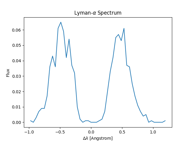
Since the output is just HDF5 files, you can plot the spectrum with a few lines of Python:
import h5py
import numpy as np
import matplotlib.pyplot as plt

with h5py.File("output/original/data.h5", "r") as f:
    dlambda = f["dlambda"][:]
    weight = f["weight"][:]

hist, bin_edges = np.histogram(dlambda, bins=50, weights=weight)
bin_centers = 0.5 * (bin_edges[:-1] + bin_edges[1:])

fig, ax = plt.subplots(figsize=(8, 5))
ax.step(bin_centers, hist, where="mid")
ax.set_xlabel(r"$\Delta\lambda$ [$\AA$]")
ax.set_ylabel("Flux [arbitrary]")
ax.set_title(r"Lyman-$\alpha$ Spectrum")
fig.tight_layout()
fig.savefig("spectrum.png", dpi=200)
plt.show()
Option B: Using thor-tools CLI
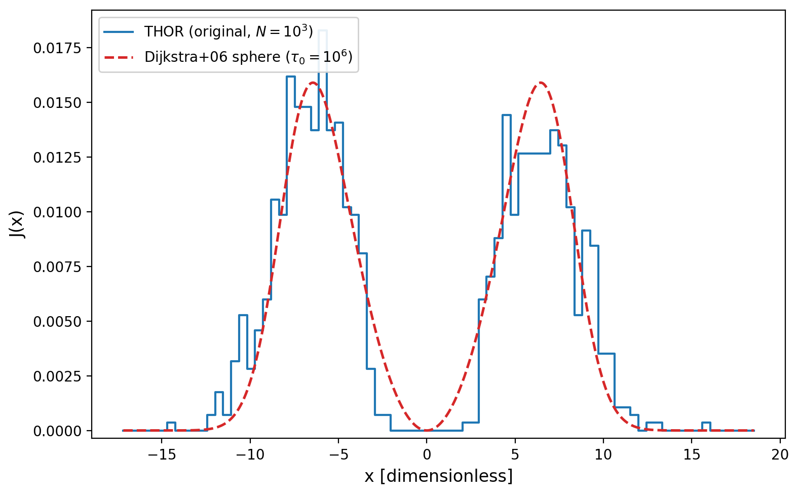
With the THOR Python packages installed (see Python Packages), plot the spectrum in one command:
This histograms escaped photons in dimensionless frequency and overlays the Dijkstra+06 static-sphere analytic solution.
To plot in wavelength space, save data, or customize binning:
# Plot in Angstrom instead of dimensionless frequency
thor-tools mcrt spectrum plot my_first_sim.yaml --xaxis dlambda

# Save spectrum data as .npz for further analysis
thor-tools mcrt spectrum plot my_first_sim.yaml --save-data -o results/

# More bins, custom range
thor-tools mcrt spectrum plot my_first_sim.yaml --nbins 100 --range "-20,20"
See thor-tools mcrt spectrum plot --help for all options.
Next Steps
- Configuration Reference - All available options
- Datasets - Detailed dataset documentation
- Cookbook - More complex setups