Coherence Length

The tracer operator is a powerful tool to trace out spatial relationships, such as the coherence of field lines. It logs field properties along ray trajectories, where both the trajectory (e.g. straight or following a vector field) and the segmentation of what gets recorded (e.g. every cell or longer stretches defined by a closing rule) are configurable.

Here we show how this works for investigating coherence lengths: with close_rule: angle_threshold each ray is cut into stretches of aligned field direction, so the segment lengths are the coherence lengths, and each segment can also carry the weighted mean of any field, e.g. the mean |B| of every coherent stretch. The example uses the magnetic and velocity field of a TNG50-4 (z=0) snapshot, in three steps: straight versus field-aligned rays on the magnetic field, field-aligned rays following the velocity versus the magnetic field, and a random ray source with pooled 1D statistics.

For intuition, here are such trajectories in motion: rays released from a camera plane follow the local magnetic field direction through the box. How far a trajectory keeps pointing the same way is the coherence length.

The fields at a glance

Before measuring anything, look at the two fields in the plane the camera fires from (sampled with the tracer itself: straight rays, close_rule: every_cell and a tiny dist_max, so each ray's first segment holds its entry cell's field values):

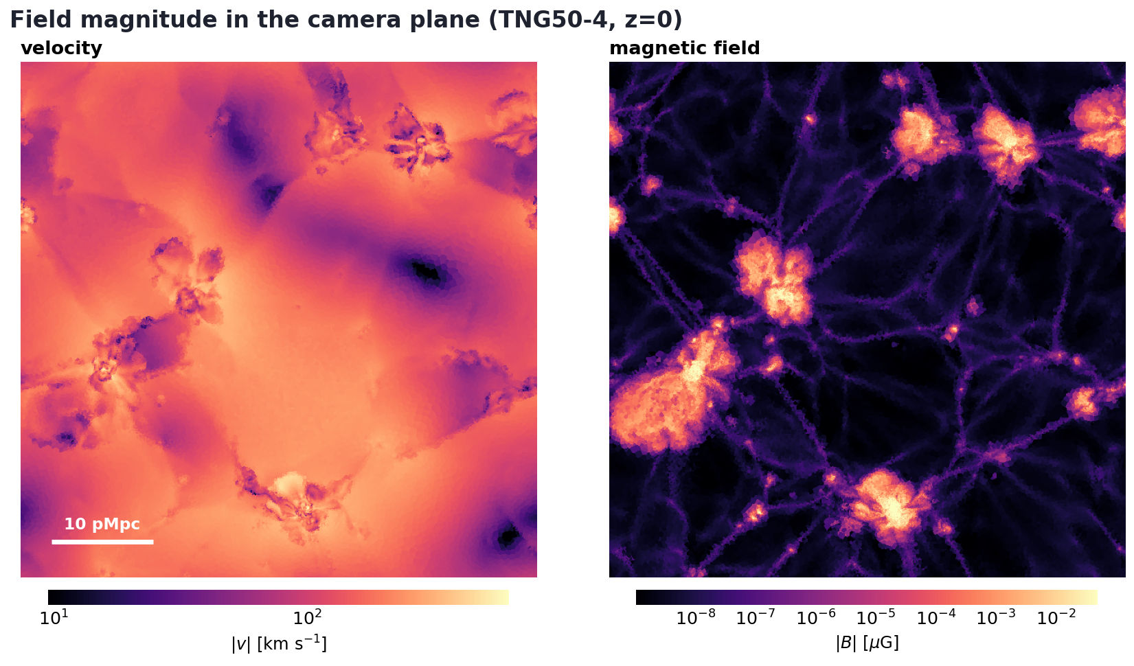
Magnitude maps show where the fields are strong, but not where they point. Since direction is what this page is about, color the same plane by it instead. Hue encodes the in-image angle (the wheel in each panel shows the mapping); gray means the field points along the line of sight:

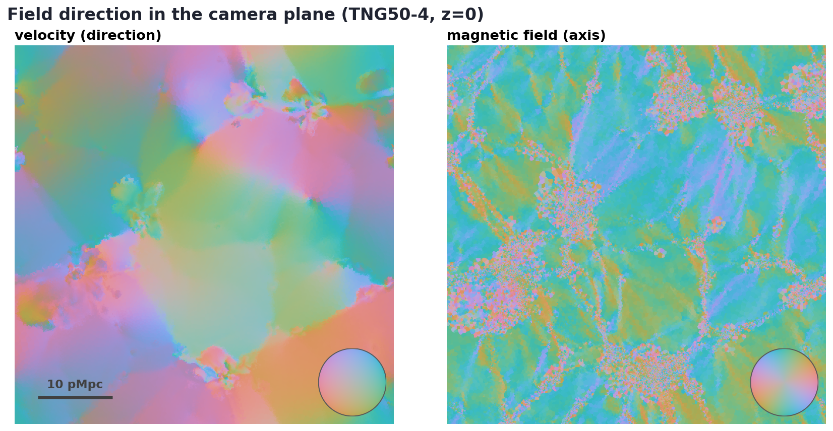
The velocity direction forms large single-hue patches: coherent bulk flows converging onto the collapsing structures. The magnetic field organizes on visibly smaller scales, fragmenting wherever the magnitude map shows structure (B carries no arrowhead, so the right panel doubles the hue angle: antiparallel directions share a color). Both maps show the direction at isolated points only. How far does the field keep pointing the same way along a path through the volume? That distance is the coherence length, and the tracer operator measures it directly.

How it works

Each ray samples direction_field cell-by-cell (where the rays start is up to the ray source: a camera plane, random points, ...). A segment opens at the first cell where |v| ≥ min_field_magnitude and stores that cell's direction as the seed. The segment grows while the local direction stays within angle_threshold degrees of the reference (see Angle reference). The first cell that exceeds the threshold closes the segment and starts a new one seeded from the new direction. Closing a segment records its path length and, with the weighted_mean accumulator, the mean of the traced field over the segment. Cells below min_field_magnitude are treated as nulls: the ray coasts through with frozen direction; they don't contribute and they don't terminate the running segment.

Two accumulators support the angle_threshold close rule:

• accumulator: weighted_mean with weight: none: each segment records its path length plus the length-weighted (spatial) mean of every entry in fields. Use this unless you need the exact legacy output; one run gives you the coherence lengths and the field statistics per coherent stretch.
• accumulator: length_only: records only the segment length (bit-identical to the legacy coherencelength operator output).

Straight vs field-aligned: the magnetic field

propagation_mode controls how each ray traverses the volume:

• straight (default): rays keep their initial direction (the camera view direction, or whatever the ray source assigned). The coherence length measures how far the field stays aligned along a straight sight line.
• field_aligned: at every cell crossing, the ray's direction is reset to the unit vector of direction_field at the new cell. The ray itself becomes a streamline (field line), and the coherence length measures how far that streamline's tangent stays aligned with its starting direction.

The camera fires an orthogonal grid of rays across the snapshot to map the coherence of MagneticField. direction_field: MagneticField tells the operator to segment on the direction of MagneticFieldX/Y/Z, and fields: [MagneticFieldMagnitude] additionally records the mean |B| per segment. We use angle_threshold: 30° as the fiducial value, inside the useful range: tight thresholds (≲15°) approach the cell-to-cell direction noise of the mesh, while at the loose 90° extreme (a segment ends only when the field flips into the opposite hemisphere) a large fraction of rays never break at all and only yield lower bounds.

dataset_type: 'pointcloud_voronoi'
driver_type: 'raytracer'
device: "cpu-openmp"

pointcloud_voronoi:
  hilbert_bits: 8
  mesh_cache_mode: "auto"
  loader: gadget
  gadget:
    path: /path/to/snapdir_099
    fields:
      - PositionX
      - PositionY
      - PositionZ
      - Density
      - MagneticFieldX
      - MagneticFieldY
      - MagneticFieldZ

raytracer:
  dist_max: 1.1
  min_step: 0
  max_step: 1.0e-2
  outputpath: ./coherence_straight.zr
  overwrite: true
  operators:
    tracers:
      mode: manual
      view: orthogonal
      position: [0.01, 0.5, 0.5]
      direction: [1.0, 0.0, 0.0]
      up: [0.0, 0.0, 1.0]
      npixels: [640, 640]
      widths: [0.98, 0.98]
      fields: [MagneticFieldMagnitude]   # mean |B| per segment
      close_rule: angle_threshold
      accumulator: weighted_mean
      weight: none                       # length-weighted (spatial) mean
      angle_threshold: 30.0
      angle_reference: cumulative    # see "Angle reference" below
      direction_field: MagneticField
      min_field_magnitude: 1.0e-10
      max_segments_per_ray: 1000

MagneticFieldMagnitude is a derived field; listing it under the tracer's fields: is enough, and the dataset materializes it from the loaded MagneticFieldX/Y/Z. max_segments_per_ray sizes the initial per-ray segment buffer. Rays that exceed it trigger a (logged) buffer-grow pass, so undersizing it costs time, not segments.

For the field-aligned variant, set pbc: true at the raytracer: level and add to the tracer block:

          propagation_mode: field_aligned
          direction_field: MagneticField
          flip_anti_parallel: true     # follow the field axis through reversals
          min_segment_length: 1.0e-6   # drop zero-length face-bounce artifacts

In field_aligned mode the configured ray direction only seeds the trajectory; the field determines the actual path. flip_anti_parallel controls what happens when the new cell's field direction points backward relative to the ray (negative dot product): false (default) treats the reversal as a stagnation point and ends the ray there; true negates the adopted direction so the ray U-turns and keeps following the field axis through the reversal.

With pbc: true a field line continues through the periodic faces instead of being truncated there; dist_max then caps its total length. The straight config deliberately leaves pbc off: a straight ray re-traces the same cells after a periodic wrap, so extending it past one box length only duplicates segments.

min_segment_length (box units) discards segments below the cut as they close. Where the direction field reverses across a cell face, a field-aligned ray can bounce on the face and log zero-length segments before moving on; a cut far below the cell scale (here ~35 pc) removes these artifacts and nothing else.

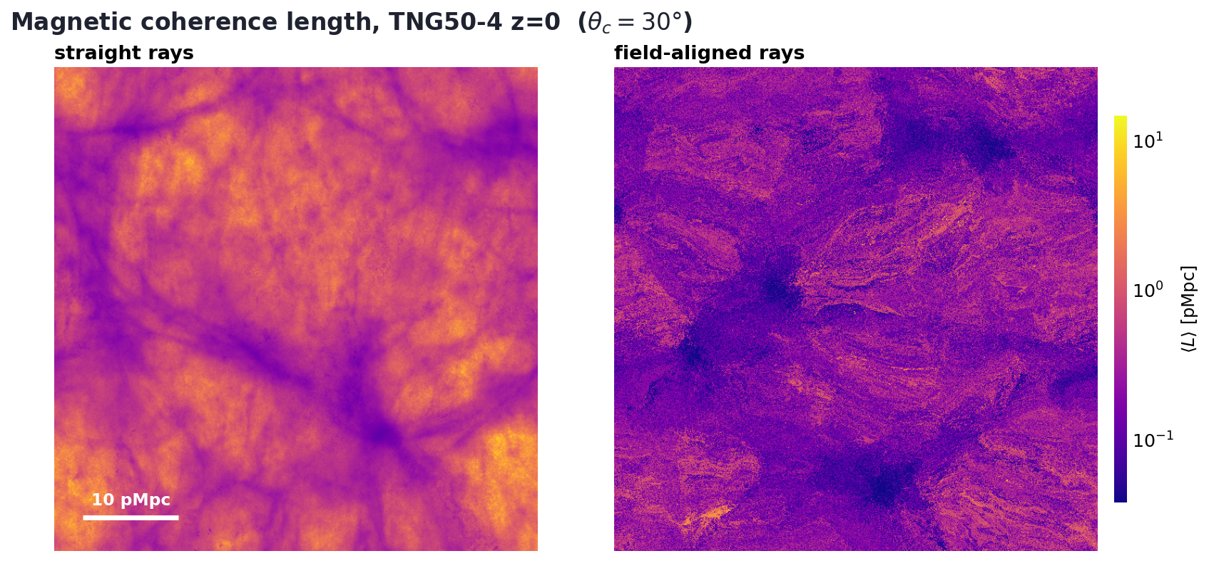
Straight rays (left) measure the apparent coherence seen by a fixed observer's sight line: long in quiet large-scale-structure regions, short where the sight line crosses collapsed objects. Field-aligned rays (right) measure the field line's own persistence (its curvature length), the natural coherence scale for problems that care about transport along field lines, e.g. cosmic-ray confinement. Adjacent entry pixels can feed into entirely different field-line paths, which gives the right panel its streaky texture.

Field-aligned: velocity vs magnetic field

Any vector field carried by the dataset can drive the propagation. Switching the field-aligned run from B to the gas velocity takes two changes in the tracer block (plus loading VelocityX/Y/Z instead of the B components):

          fields: [VelocityMagnitude]
          direction_field: velocity

Both runs set flip_anti_parallel: true, so both maps measure axis coherence: rays follow the field's orientation through sign reversals. For B that is the natural choice, since a field line has no arrowhead. Velocity does carry a meaningful sign, so with the default false a ray ends where the flow reverses — a genuine stagnation point. We set true here for a clean like-for-like comparison with B (both follow the field axis through reversals).

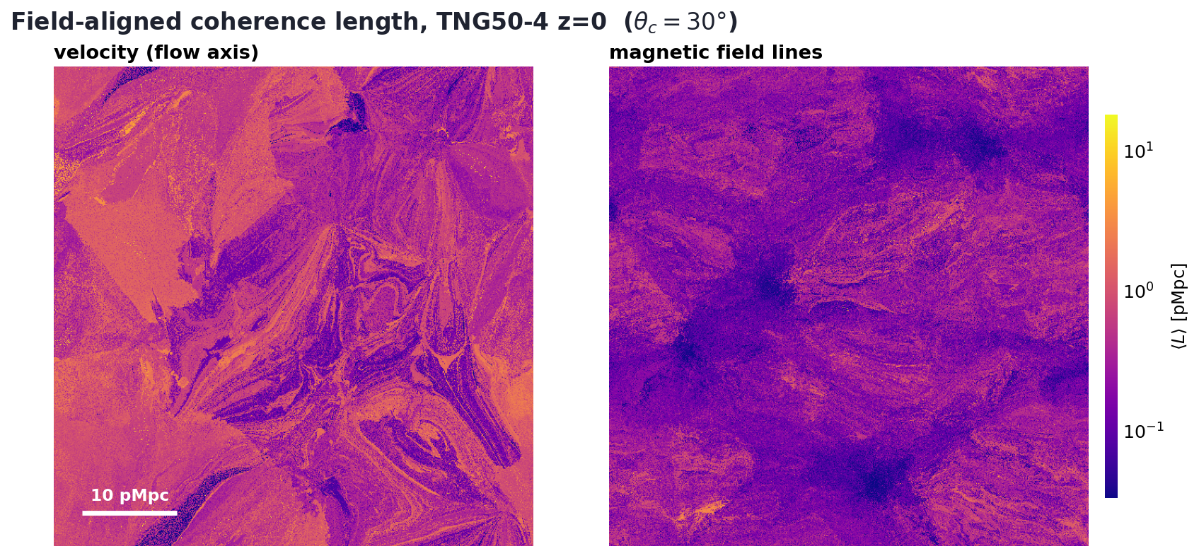
The two fields organize on very different scales: large-scale flows stay ordered over tens of pMpc, while the magnetic field decorrelates on far smaller scales nearly everywhere. Rays that never break twice have no interior segments to average; rather than leaving those pixels blank, the map fills them with the ray's traced path (~57 pMpc here). The measurement saturated, so this is a lower bound on the coherence length (the flat yellow regions).

Angle reference: cumulative vs continuous

angle_reference controls what the per-cell field direction is compared against to decide when a segment ends:

• cumulative (default): compare each cell's direction against the segment's seed direction (the cell where the segment started). A segment ends only when the field has drifted by more than angle_threshold from where it began. Captures slow rotation over many cells.
• continuous: compare each cell's direction against the previous cell's direction. A segment ends only at an abrupt turn larger than angle_threshold between adjacent cells. Slow rotation (small per-cell increments below threshold) never ends the segment, even if the field rotates 180° over the box.

How continuous mode segments one ray, cell by cell (drawn for a field_aligned ray, so the trajectory adopts each cell's field direction and kinks at every face):

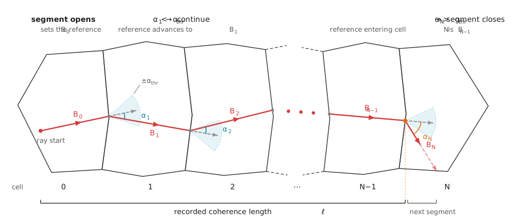
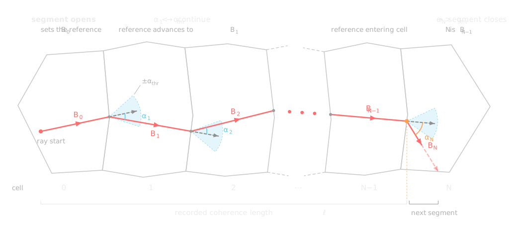
The breaking cell is not lost: it opens the next segment (drawn faint — its path no longer counts toward the recorded ℓ), and in continuous mode its direction is also the reference its successor is measured against. For a straight ray the same segmentation applies, only the trajectory stays a straight line while the sampled directions turn.

Under cumulative the dashed reference stays frozen at the segment's seed direction B₀ instead of advancing cell by cell — every cell is compared against where the segment started:

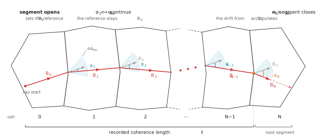
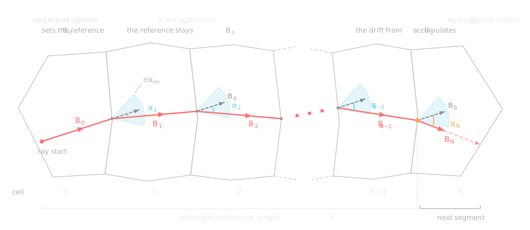
Note that here no single turn is sharp — the closing turn is only 12°, so continuous mode would trace straight on — but the drift from B₀ (13°, 23°, …, 27°, 39°) accumulates past the threshold. That is the practical difference: cumulative breaks on slow rotation over many cells, continuous only on abrupt cell-to-cell turns.

The difference between the two is a diagnostic in itself: on the field-aligned runs above, switching from cumulative to continuous removes far more velocity-field breaks (gradual flow curvature) than magnetic-field breaks (abrupt small-scale tangles).

Random ray source and pooled statistics

The camera plane is just one way to seed rays. Any ray source works; random_uniform seeds rays uniformly throughout the volume with isotropic initial orientations (for field-aligned rays, the initial direction only picks which way along the field line the ray heads). Replace the camera keys with:

        tracers:
          ray_source:
            type: random_uniform
            n_rays: 200000
            direction_distribution: isotropic
            seed: 42
          # ... same tracer keys as before ...

The output layout is Scatter: per-ray arrays without pixel ordering, so there is no map; pooled 1D statistics are the natural product (the origins array still records each seed position if you need spatial context). Volume seeding is also the more natural ensemble for global field-line statistics: a camera plane samples field lines by where they pierce one box face, while random seeding weights them by volume.

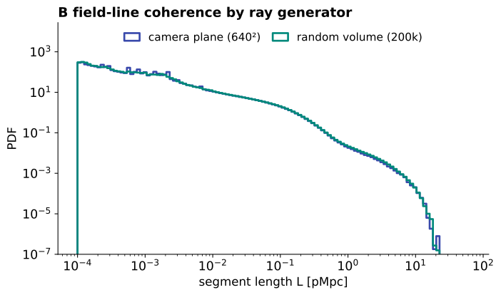
The two seedings agree closely in the shape of the distribution, so the coherence-length statistics are largely robust to the ray source. As the volume-weighting argument above anticipates, the random sample is the smoother and more representative of the two: it draws many independent field lines, whereas the finite camera plane samples a correlated subset (the lines that pierce one face) and traces a visibly noisier curve — most apparent at the short-segment end.

Reading the Output

The tracer writes one zarr group per traced field (lower-cased name) with flat, compacted per-segment arrays: ray i's segments occupy [offsets[i], offsets[i+1]), and the last ray runs to the end of the array.

The table shows the weighted_mean layout used here. With accumulator: length_only, the segment length is written to contributions instead and lengths stays zero.

n_rays is set by the ray source: npx·npy for a camera plane, n_rays for random_uniform. For a camera plane, ray order is pixel order, so per-ray quantities reshape to (npy, npx) maps.

import numpy as np
import zarr

g = zarr.open("coherence_straight.zr", mode="r")["tracers/magneticfieldmagnitude"]
lengths = g["lengths"][:]                  # segment lengths (box units)
mean_b  = g["contributions"][:]            # mean |B| per segment (field units)
offsets = g["offsets"][:].astype(np.int64)

per_ray = np.split(lengths, offsets[1:])   # one array of segments per ray

Slicing each ray's segments with [1:-1] drops the cut-short first and last segment (see note above). Because each segment also carries its mean |B|, the field-strength / coherence-length correlation comes from the same single run:

import matplotlib.pyplot as plt

box = 51.7  # physical box size in Mpc (tracer lengths are in box units)
pooled   = np.concatenate([s[1:-1] for s in per_ray]) * box
pooled_b = np.concatenate([b[1:-1] for b in np.split(mean_b, offsets[1:])])
plt.hexbin(pooled, pooled_b, xscale="log", yscale="log", mincnt=1)

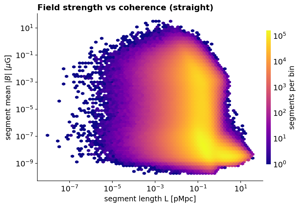
Per-segment field statistics against coherence length is a product the legacy operator could not produce; here, long coherent stretches are confined to the weakly magnetized volume.

Migrating from the coherencelength operator

Rename vector_field to direction_field, add close_rule: angle_threshold, and pick an accumulator (length_only reproduces the legacy output exactly; weighted_mean is the better default). Most other keys carry over unchanged. The main gotchas: the output moves to tracers/<field>/ as per-segment arrays (no per-pixel mean map; compute it as shown above), and segment lengths are in normalized box units instead of cm.

See Also

• Ray Tracer Driver: the full tracer configuration table (stop rules, multi-field tracing, per-cell trajectory dumps), camera modes, view types, shared ray-tracer parameters.
• Datasets Reference: pointcloud_voronoi configuration.