Sightline Absorption

The sightline operator turns a ray through the box into an absorption spectrum. Along each ray it records the traversed gas cells (density, temperature, velocity, …) and integrates them into an optical-depth profile τ(λ) by summing a Doppler-shifted Voigt line for every cell. It's where absorption work in THOR now lives, replacing the older absorptiongrids operator.

This page walks one sightline through a structured field (four neutral-hydrogen clumps at different line-of-sight velocities, the canonical QSO-absorber picture), from the raw cell dump to a mock observed Lyα spectrum.

For intuition, here is the integration in motion: as the ray crosses each clump, that clump deposits a Voigt line into the running optical depth, on the opposite side of line centre to its velocity (gas moving toward the observer is blueshifted).

Left: neutral-hydrogen density along the ray, with a marker at the cell currently being integrated. Right: the optical depth accumulated so far. Each clump adds a Voigt trough at the velocity set by its line-of-sight motion.

The sightline at a glance

Before integrating anything, look at what the operator records cell-by-cell along the ray. These are the operator's own per-cell arrays (one entry per traversed cell), the raw material the τ integration consumes:

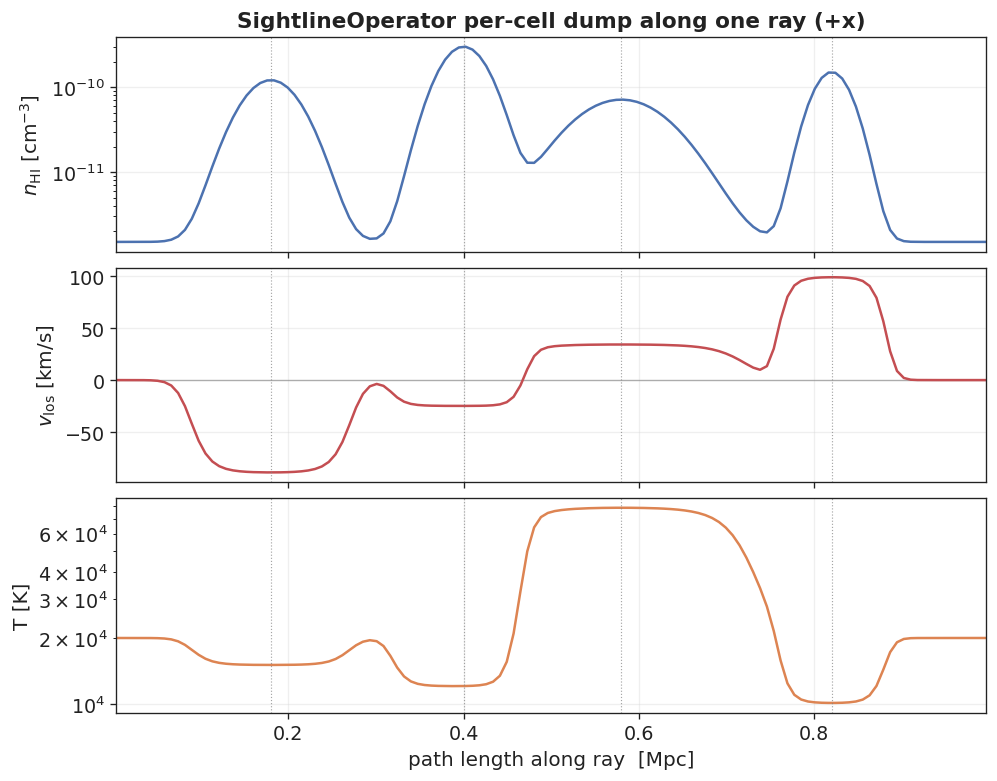
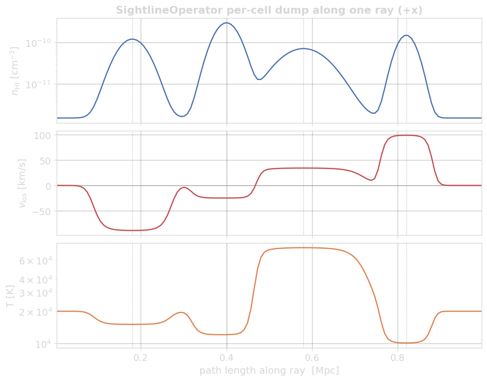
Four density clumps sit at different positions along the ray. Each carries its own line-of-sight velocity (middle panel): two receding (v_los < 0) and two approaching (v_los > 0). The third clump is hot (intrinsic T = 8 × 10⁴ K; the density-weighted curve peaks near 7 × 10⁴ K), which will make its line thermally broad. The velocity maps each clump to a wavelength (with a sign flip explained below: approaching gas absorbs blueward), and the temperature sets each line's width.

How it works

For each spectral bin i (wavelength λ_i, frequency ν_i = c/λ_i) the operator sums over every cell the ray crossed:

\[\tau(\lambda_i) = \sum_{\rm cells} n_{\rm ion}\, \mathrm{d}l \; \sigma_{\rm Voigt}\!\big(\lambda_i;\, T,\, v_{\rm los}\big)\]

with three pieces per cell:

Column n_ion · dl: the ion number density times the path length through the cell. For Lyα that ion is H I; the tau: block routes the relevant density field to each line.
Line centre (the Doppler shift). The ray direction points source → observer, so a cell whose gas moves toward the observer (v_los > 0 along the ray) is blueshifted: its line lands at λ < λ₀, while gas receding from the observer is redshifted to λ > λ₀. (THOR composes this peculiar shift relativistically, including transverse time dilation, with the cosmological redshift into a single effective shift λ₀(1 + z_eff); with Hubble flow off and a single snapshot it reduces to the simple Doppler term.)
Line width (the Voigt profile). The Doppler parameter b = √(2kT/(A m_u) + v_turb²) sets the Gaussian core, where A is the atomic mass number, m_u the atomic mass unit, and v_turb an optional turbulent broadening term; the line's natural width sets the Lorentzian wings. Hot or turbulent cells give broad, shallow lines; cold cells give narrow, deep ones. Narrow lines that fall below the bin width are integrated within the bin so τ is not under-sampled.

Because τ is a sum over cells, it is additive: each clump's contribution is independent and they stack. Splitting the total by clump shows exactly where each ends up:

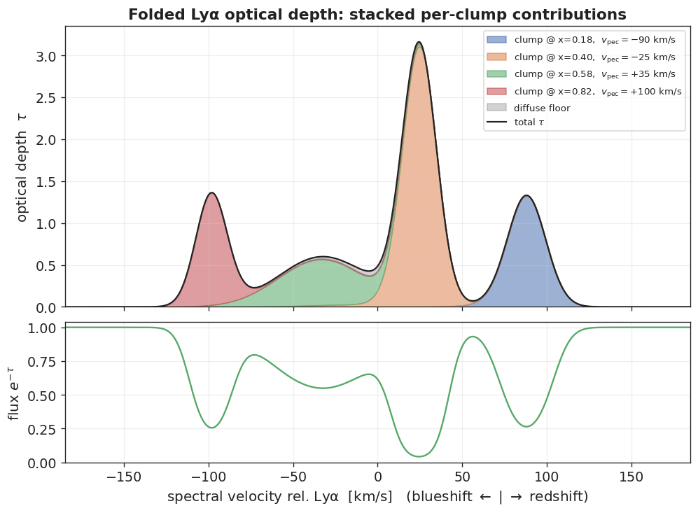
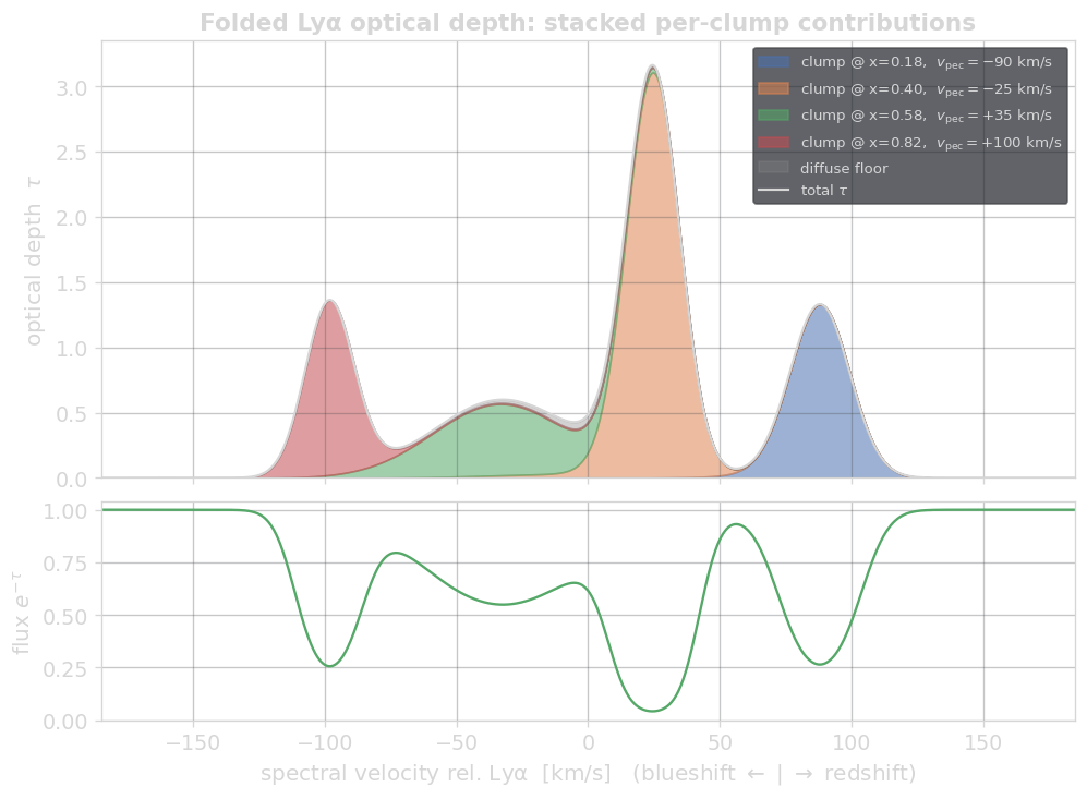
Read the velocity convention off the arrows. The clump approaching at +100 km/s (red) produces the trough at −100 km/s (blueshift); the clump receding at −90 km/s (blue) lands at +90 km/s (redshift). The hot clump (green) is broad and shallow at the same column, its thermal width spreading the absorption out. The strongest clump (orange) is mildly saturated (τ ≈ 3, its flux trough bottoms near zero). A faint diffuse floor fills the gaps. This velocity → wavelength mapping is the whole point of a sightline: the absorption profile is a velocity-space tomogram of the gas the ray crossed.

Peculiar velocity vs. Hubble flow

This example is a single static box, so the velocity spread comes entirely from the clumps' peculiar line-of-sight velocities (Hubble flow is off). In a real cosmological sightline the separation between absorbers at different distances is dominated instead by Hubble flow (distance maps to redshift), with peculiar velocities as perturbations on top; the peculiar velocities used here effectively stand in for that. THOR models the cosmological case directly via raytracer.hubble_flow and hubble_mode; see the Ray Tracer Driver.

Full configuration

The ray traces a structured pregridded box; the tau: block integrates the Lyα profile while the cell-field passes dump the per-cell arrays into the same store.

sightline_clumps.yaml

dataset_type: 'unigrid'
driver_type: 'raytracer'
device: 'cpu'

unigrid:
  ngrid: 128
  loader: gadget
  gadget:
    path: './dummy'                          # placeholder; required even for pregridded loads
    pregridded_path: './grid_clumps.hdf5'    # HI clumps + velocity field
    boxsize: 3.0857e24                        # 1 Mpc
    domain_consistency_check: false

raytracer:
  max_step: 1.0
  outputpath: './thor_sightline_clumps.zr'
  overwrite: true
  operators:
    sightlines:
      rays:
        - { id: 0, start: [0.0, 0.5, 0.5], end: [1.0, 0.5, 0.5] }
      tau:
        linename: 'Lya'
        edge_left: -0.75      # ≈ -185 km/s at Lyα 1215.67 Å
        edge_right: 0.75      # ≈ +185 km/s
        nbins: 1024

edge_left/edge_right are offsets in Å from the line centre; nbins sets the spectral resolution. Many rays at once come from a ray source (camera_plane, camera_healpix, random_uniform) instead of a hand-listed rays: list. Multi-line spectra, per-line ion-density routing, and hubble_flow / hubble_mode are documented in the Ray Tracer Driver page.

Observer realism

The integrated τ is the physical prediction. To compare with a real spectrograph, the thor.absorption Python package layers on observer effects, each step returning self so they chain:

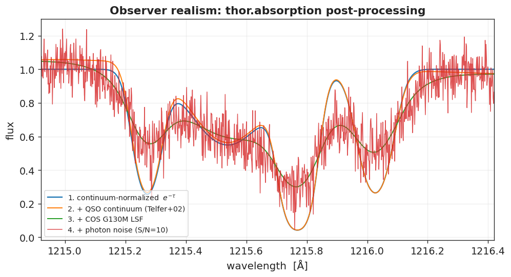
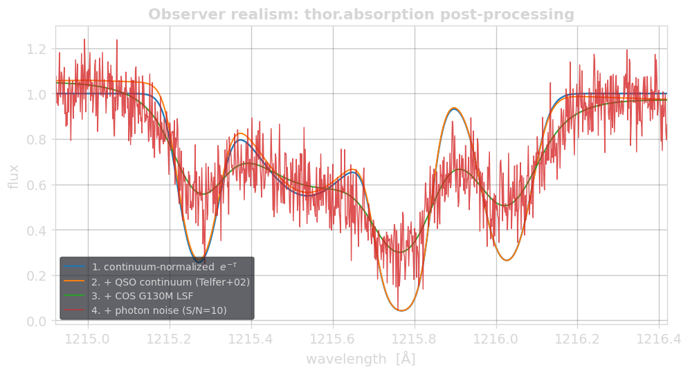
from thor.absorption import Sightline, Instrument, SpectrumPostProcessor

spec = Sightline("thor_sightline_clumps.zr").spectrum(ray_id=0)   # (lam, tau)
pp = (
    SpectrumPostProcessor(spec)
    .add_qso("qso_telfer2002")        # QSO continuum
    .add_mw_fg("mw_fg_danforth2016")  # Milky-Way foreground (optional)
    .apply_lsf(Instrument("COS-G130M"))
    .add_noise(snr=10, seed=7)
)
pp.save("mock_spectrum.fits")

At this narrow Lyα window the COS LSF is far smaller than the line widths, so it barely smooths the profile; photon noise dominates the difference. Over a broad multi-line spectrum the LSF and QSO-continuum shape matter much more.

Reading the output

SightlineOperator writes a flat/dense layout under sightlines/<savename>/ (default default): a shared wavelength grid plus a dense τ array, with optional per-cell field arrays addressed by a cell_offsets index array. Because each ray crosses a different number of cells, the per-cell fields are stored as one flat array indexed by offsets (the compressed-sparse-row (CSR) layout): ray i's cells occupy [cell_offsets[i], cell_offsets[i+1]), and the last ray runs to the end of the array.

Key	Shape	Description
`sightlines/<name>/lam`	`(nbins,)`	shared bin-centred wavelength grid [Å]
`sightlines/<name>/tau`	`(nray, nbins)`	integrated optical depth per ray
`sightlines/<name>/ray_id`	`(nray,)`	ray identifiers
`sightlines/<name>/start`, `…/end`	`(nray, 3)`	ray endpoints
`sightlines/<name>/cell_offsets`	`(nray+1,)`	offset index into the per-cell arrays (CSR-style)
`sightlines/<name>/{density,temperature,velocity_x,…,dl}`	`(N_cells_total,)`	flat per-cell fields

The Sightline loader resolves all of this (the ray_id → row lookup, the CSR slicing, and the (lam, tau) Spectrum), so analysis code never indexes the raw arrays by hand:

import numpy as np
from thor.absorption import Sightline

sl = Sightline("thor_sightline_clumps.zr")
lam, tau = sl.lam, sl.tau(ray_id=0)     # integrated spectrum
cells = sl.fields(ray_id=0)             # {'density','temperature','velocity_x',...}
dl = sl.dl(ray_id=0)                    # per-cell path length (box units)

# velocity-space view, matching the convention above
v_obs = (lam - 1215.67) / 1215.67 * 2.99792458e5   # km/s; blueshift < 0

Trident interoperability

THOR can stand in for Trident for sightline absorption: it integrates τ directly on the native simulation mesh (GPU-accelerated via SYCL), so the thor.absorption pipeline above is usually all you need. When you specifically want Trident's background source spectra (QSO continuum, Milky-Way foreground) or its instrument models, to_trident_spectrum_generator hands you a live trident.SpectrumGenerator with THOR's τ already loaded. From there it is plain Trident, and every normal Trident spectrum method works on the returned object:

from thor.absorption import Sightline, to_trident_spectrum_generator

spec = Sightline("thor_sightline_clumps.zr").spectrum(ray_id=0)
sg = to_trident_spectrum_generator(spec)   # a trident.SpectrumGenerator, τ already loaded

# ...from here, just use Trident as usual:
sg.add_qso_spectrum()              # Trident's QSO background
sg.add_milky_way_foreground()      # Trident's MW foreground
sg.apply_lsf()                     # Trident instrument model
sg.add_gaussian_noise(30)
sg.save_spectrum("spectrum.h5")    # or sg.plot_spectrum("spectrum.png")

Trident is an optional, self-installed dependency (pip install trident); THOR does not bundle it.

Examples

Three worked examples take the same operator from the toy clumps above to a cosmological box: a Lyα forest through TNG50-4, a mock quasar spectrum built from a long skewer, and metal-line CGM absorption through an AGORA galaxy.

A real Lyα forest: TNG50-4

The same operator scales straight to a cosmological box. Here it traces a 512×512 grid of sightlines along +x through the full TNG50-4 snapshot at z = 0 (35 Mpc/h, ≈ 51.7 pMpc, ~18.5 million Voronoi gas cells). The neutral-hydrogen density comes straight from the snapshot's NeutralHydrogenAbundance (THOR derives HIdensity natively, so HI needs no Cloudy table), and Hubble flow is on, so every sightline yields a genuine Lyα forest.

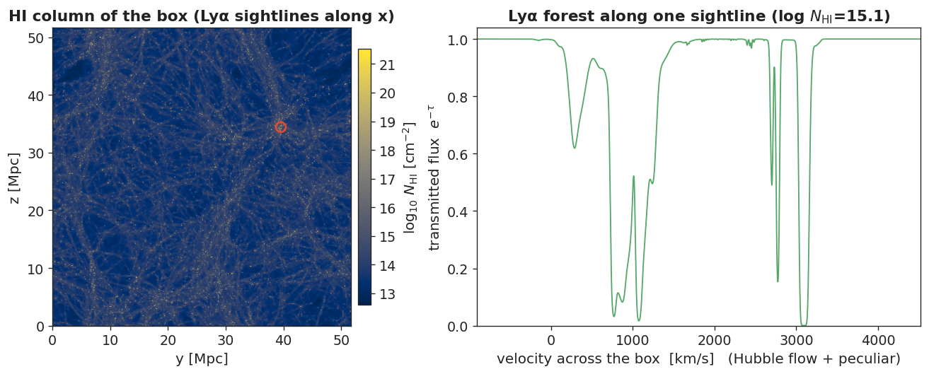
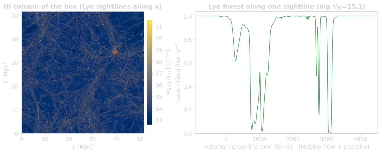
Left: the HI column of every sightline (Σ n_HI · dl) reshaped to the camera grid, the cosmic web in N_HI, with bright high-column systems (Lyman-limit and damped-Lyα absorbers in collapsed halos) threading a diffuse IGM. Right: the transmitted flux along the circled sightline. This is the picture the toy example only stood in for: absorbers at different distances along the box appear at different velocities (distance maps to recession velocity through Hubble flow), from shallow IGM ripples to a saturated system, spread across the ~3500 km/s the box subtends.

Nothing about the operator changed, only the dataset and the density routing:

TNG50-4 configuration (excerpt)

dataset_type: 'pointcloud_voronoi'        # build a Voronoi mesh on the gas cells
pointcloud_voronoi:
  construction:
    ghost_thickness: 0.1                  # periodic ghost shell as a box fraction; the
                                          # default 0.51 ≈ full replication and OOMs at 18.5M cells
  loader: gadget
  gadget:
    path: /path/to/TNG50-4_snapshot
    fields: ["PositionX", "PositionY", "PositionZ", "Temperature", "Density",
             "VelocityX", "VelocityY", "VelocityZ", "HIdensity"]
raytracer:
  pbc: true                               # true periodic Voronoi
  hubble_flow: 67.74                       # H0 [km/s/Mpc] = h·100 at z=0 → the forest
  operators:
    sightlines:
      ray_source: { type: camera_plane, npixels: [512, 512], direction: [1.0, 0.0, 0.0], length: 1.0 }
      fields: ["HIdensity"]
      tau:
        lines: ['Lya']
        line_density_fields: { Lya: HIdensity }   # integrate n_HI, not the gas mass density
        lambda_min: 1212.0
        lambda_max: 1234.0
        nbins: 2048

HIdensity is derived from the snapshot's neutral fraction; line_density_fields routes the Lyα deposit to it (the default integrates the gas mass density, which is wrong for a line). For metal lines (O VI, Mg II, …) point cloudy.ion_table_path at a Cloudy ion table and route e.g. OVI: cloudydensity_OVI.

Building a mock QSO spectrum

A single box crossing samples a short path. To synthesize a full quasar sightline, i.e. a long Lyα forest blueward of the QSO's Lyα emission, fire the ray at an oblique angle and let it wrap through the periodic box many times (length: 10 box units, pbc: true). With an incommensurate direction each wrap threads fresh structure, so the ray accumulates a long forest spanning the box's Hubble flow (~10 × 3500 km/s, i.e. Δz ≈ 0.12 here). Integrating the Lyman series (Lyα–Lyε) plus the Lyman continuum in one pass gives the Lyα forest, the Lyβ forest, and the Lyman-limit break together. Treat the far end as a quasar at that redshift and multiply the forest transmission exp(−τ) by the qso_telfer2002 QSO continuum (redshifted to z_qso):

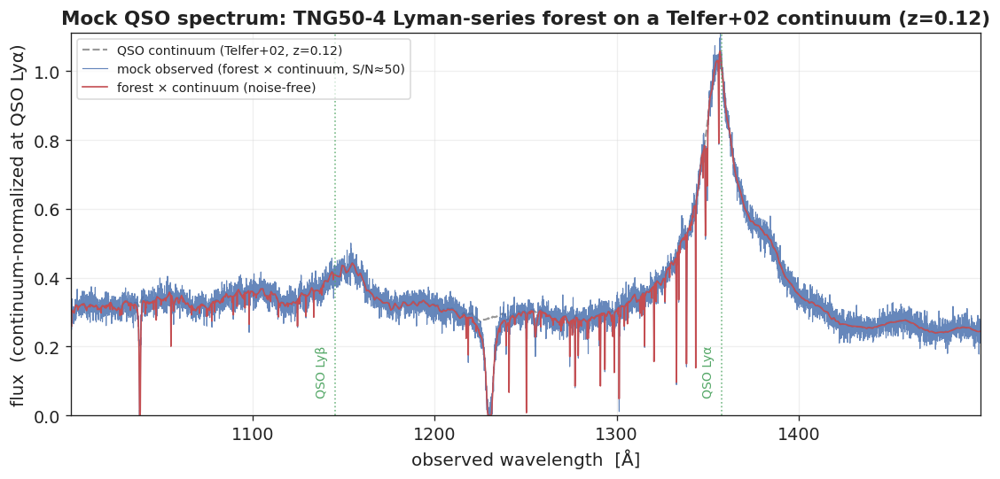
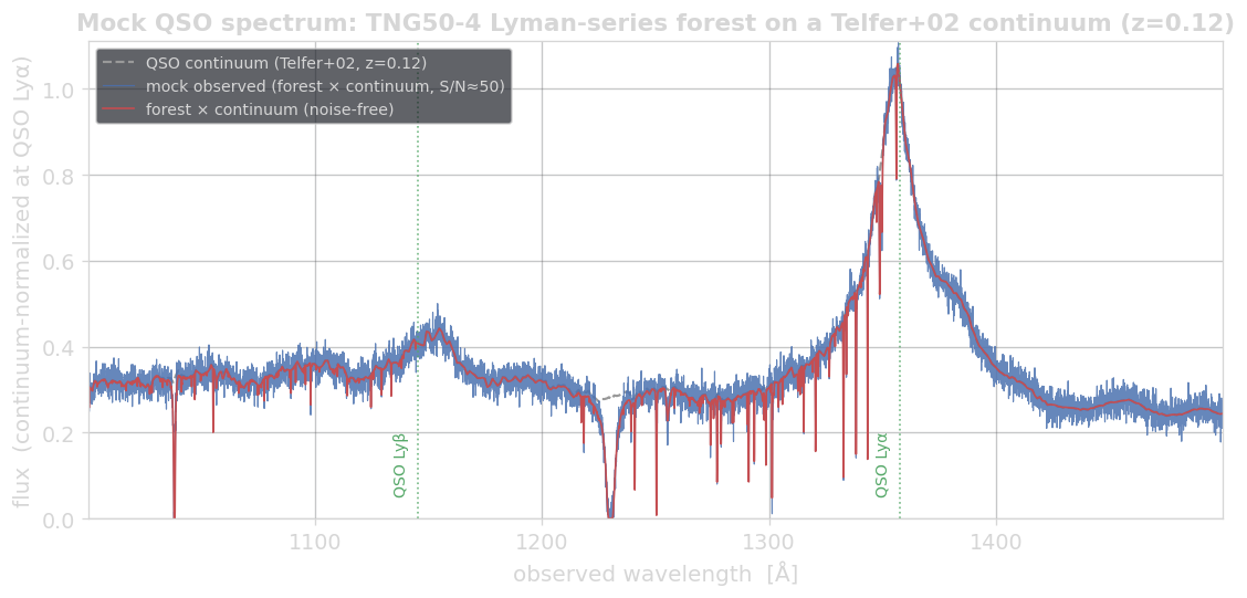
Redward of the QSO Lyα emission peak (~1358 Å) the spectrum is bare continuum. Blueward lies the Lyα forest, and blueward of the QSO Lyβ peak (~1147 Å) the same absorbers reappear as the weaker Lyβ forest.

Long-skewer + QSO configuration (excerpt)

raytracer:
  pbc: true
  hubble_flow: 67.74
  operators:
    sightlines:
      ray_source:
        type: camera_plane
        direction: [0.892, 0.383, 0.241]    # oblique → fresh structure on each periodic wrap
        length: 10.0                         # ~10 box crossings of forest
      fields: ["HIdensity"]
      tau:
        lines: ['Lya', 'Lyb', 'Lyc', 'Lyd', 'Lye']         # Lyman series
        line_density_fields:
          Lya: HIdensity
          Lyb: HIdensity
          Lyc: HIdensity
          Lyd: HIdensity
          Lye: HIdensity
        include_lyman_continuum: true        # Lyman-limit break
        ll_density_field: HIdensity
        lambda_min: 1000.0
        lambda_max: 1500.0
        nbins: 8192

Then overlay the QSO continuum in Python: redshift the template to the quasar's z and multiply by the forest transmission:

import numpy as np
from importlib.resources import files
from thor.absorption import Sightline

spec = Sightline("tng_qso.zr").spectrum(ray_id=7)        # (lam, tau) of the long skewer
z_qso = 0.12                                             # far end of the ray
tpl = np.loadtxt(files("thor.absorption") / "data" / "spectral_templates" / "qso_telfer2002.txt")
continuum = np.interp(spec.lam / (1 + z_qso), tpl[:, 0], tpl[:, 1])
mock_flux = continuum * np.exp(-spec.tau)               # QSO continuum × forest

(SpectrumPostProcessor.add_qso multiplies the template in the rest frame; the redshift to z_qso is the one extra step a true mock-QSO needs.)

Metal lines: CGM absorption through an AGORA galaxy

The same operator does metal-line absorption: route each line to a metal-ion density instead of n_HI. Here it traces sightlines through the circumgalactic medium of the AGORA project's z = 4 GIZMO galaxy in three standard UV metal lines — O VI (1032, 1038 Å), C IV (1548, 1551 Å) and Si IV (1394, 1403 Å).

The snapshot doesn't store these ions, so THOR derives each from a Cloudy ionization table (cloudy.ion_table_path) at load — per cell, from its density, temperature, redshift and metallicity — giving cloudydensity_OVI, cloudydensity_CIV, cloudydensity_SiIV. tau.line_density_fields then routes each line to its ion, as { Lya: HIdensity } did for hydrogen.

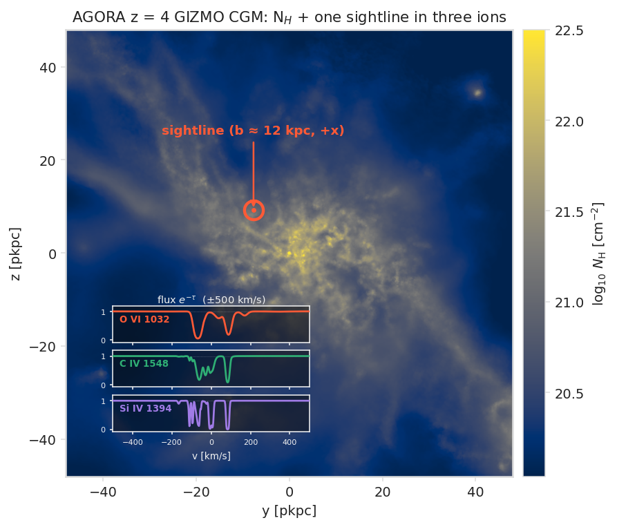
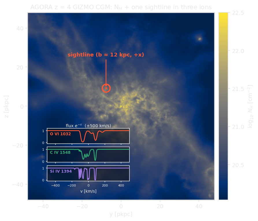
The panel is a THOR projection of the halo (total-hydrogen column here, but any field works); the marked sightline is one ray through the CGM, and its embedded spectrum is exactly what the tau: block records along it. All three ions are integrated in one pass; the configuration below sweeps an 8×8 grid of such sightlines.

AGORA CGM multi-ion configuration (excerpt)

A Voronoi mesh on the GIZMO gas cells, metal-ion densities derived from the Cloudy table at load, and an 8×8 grid of sightlines traced in all three doublets:

dataset_type: 'pointcloud_voronoi'         # Voronoi mesh on the GIZMO gas cells
pointcloud_voronoi:
  loader: gadget
  cloudy:
    enabled: true                          # derive metal-ion densities at load
    ion_table_path: /path/to/cloudy_tables/grid_ions_lg_c23.hdf5
  gadget:
    path: /path/to/agora_gizmo_z4/snapshot_152.hdf5
    fields: ["PositionX", "PositionY", "PositionZ", "Density", "Temperature",
             "Metallicity", "StarFormationRate",
             "cloudydensity_OVI", "cloudydensity_CIV", "cloudydensity_SiIV"]
    zoom_box: [[0.4823, 0.5049], [0.5080, 0.5306], [0.4918, 0.5143]]  # halo + CGM cutout
  field_filters:
    _sfr_zero:                             # drop star-forming ISM: CGM table only
      conditions: [{ field: StarFormationRate, op: "==", value: 0.0 }]
      else: zero
    cloudydensity_OVI:  { inherit: _sfr_zero }
    cloudydensity_CIV:  { inherit: _sfr_zero }
    cloudydensity_SiIV: { inherit: _sfr_zero }

raytracer:
  operators:
    sightlines:
      ray_source: { type: camera_plane, npixels: [8, 8], direction: [1.0, 0.0, 0.0], length: 1.0 }
      tau:
        lines: ["OVI 1032", "OVI 1038", "CIV 1548", "CIV 1551", "SiIV 1394", "SiIV 1403"]
        per_species: true                  # each ion on its own compact λ window
        line_density_fields:
          "OVI 1032":  cloudydensity_OVI
          "OVI 1038":  cloudydensity_OVI
          "CIV 1548":  cloudydensity_CIV
          "CIV 1551":  cloudydensity_CIV
          "SiIV 1394": cloudydensity_SiIV
          "SiIV 1403": cloudydensity_SiIV
        lambda_min: 1020.0
        lambda_max: 1560.0
        nbins: 27000                        # ~0.02 Å (~6 km/s at 1032 Å)

per_species: true writes each ion onto its own compact wavelength window (see Ray Tracer Driver). The run is cross-checked against Trident-generated spectra for the same AGORA halo.