Sightline Absorption

The sightline operator turns a ray through the box into an absorption spectrum. Along each ray it records the traversed gas cells (density, temperature, velocity, …) and integrates them into an optical-depth profile τ(λ) by summing a Doppler-shifted Voigt line for every cell. It's where absorption work in THOR now lives, replacing the older absorptiongrids operator.

This page walks one sightline through a structured field (four neutral-hydrogen clumps at different line-of-sight velocities, the canonical QSO-absorber picture), from the raw cell dump to a mock observed Lyα spectrum.

For intuition, here is the integration in motion: as the ray crosses each clump, that clump deposits a Voigt line into the running optical depth, on the opposite side of line centre to its velocity (gas moving toward the observer is blueshifted).

The sightline at a glance

Before integrating anything, look at what the operator records cell-by-cell along the ray. These are the operator's own per-cell arrays (one entry per traversed cell), the raw material the τ integration consumes:

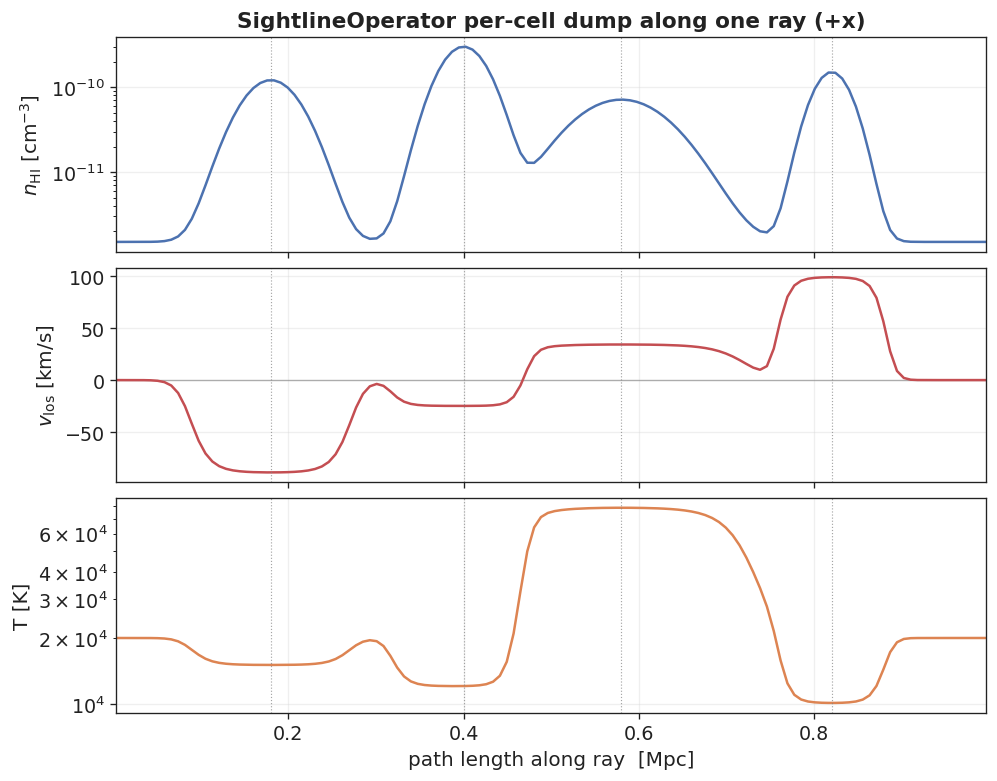
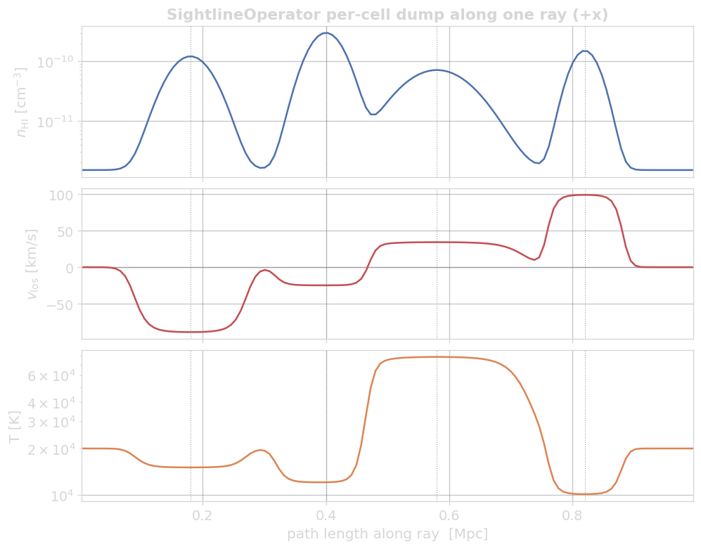
Four density clumps sit at different positions along the ray. Each carries its own line-of-sight velocity (middle panel): two receding (v_los < 0) and two approaching (v_los > 0). The third clump is hot (intrinsic T = 8 × 10⁴ K; the density-weighted curve peaks near 7 × 10⁴ K), which will make its line thermally broad. The velocity maps each clump to a wavelength (with a sign flip explained below: approaching gas absorbs blueward), and the temperature sets each line's width.

How it works

For each spectral bin i (wavelength λ_i, frequency ν_i = c/λ_i) the operator sums over every cell the ray crossed:

with three pieces per cell:

• Column n_ion · dl: the ion number density times the path length through the cell. For Lyα that ion is H I; the tau: block routes the relevant density field to each line.
• Line centre (the Doppler shift). The ray direction points source → observer, so a cell whose gas moves toward the observer (v_los > 0 along the ray) is blueshifted: its line lands at λ < λ₀, while gas receding from the observer is redshifted to λ > λ₀. (THOR composes this peculiar shift relativistically, including transverse time dilation, with the cosmological redshift into a single effective shift λ₀(1 + z_eff); with Hubble flow off and a single snapshot it reduces to the simple Doppler term.)
• Line width (the Voigt profile). The Doppler parameter b = √(2kT/(A m_u) + v_turb²) sets the Gaussian core, where A is the atomic mass number, m_u the atomic mass unit, and v_turb an optional turbulent broadening term; the line's natural width sets the Lorentzian wings. Hot or turbulent cells give broad, shallow lines; cold cells give narrow, deep ones. Narrow lines that fall below the bin width are integrated within the bin so τ is not under-sampled.

Because τ is a sum over cells, it is additive: each clump's contribution is independent and they stack. Splitting the total by clump shows exactly where each ends up:

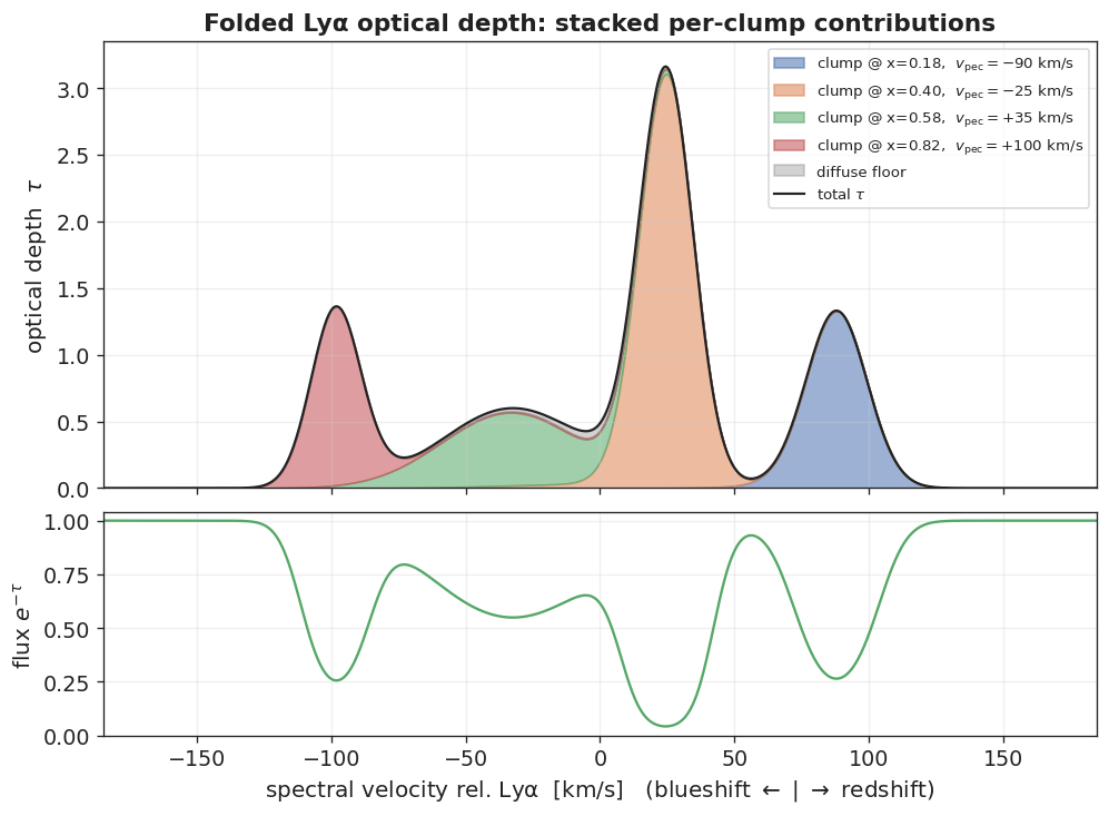
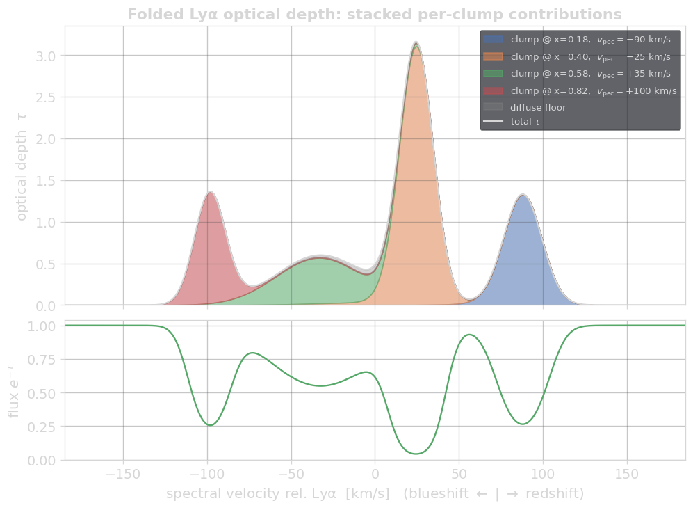
Read the velocity convention off the arrows. The clump approaching at +100 km/s (red) produces the trough at −100 km/s (blueshift); the clump receding at −90 km/s (blue) lands at +90 km/s (redshift). The hot clump (green) is broad and shallow at the same column, its thermal width spreading the absorption out. The strongest clump (orange) is mildly saturated (τ ≈ 3, its flux trough bottoms near zero). A faint diffuse floor fills the gaps. This velocity → wavelength mapping is the whole point of a sightline: the absorption profile is a velocity-space tomogram of the gas the ray crossed.

dataset_type: 'unigrid'
driver_type: 'raytracer'
device: 'cpu'

unigrid:
  ngrid: 128
  loader: gadget
  gadget:
    path: './dummy'                          # placeholder; required even for pregridded loads
    pregridded_path: './grid_clumps.hdf5'    # HI clumps + velocity field
    boxsize: 3.0857e24                        # 1 Mpc
    domain_consistency_check: false

raytracer:
  max_step: 1.0
  outputpath: './thor_sightline_clumps.zr'
  overwrite: true
  operators:
    sightlines:
      rays:
        - { id: 0, start: [0.0, 0.5, 0.5], end: [1.0, 0.5, 0.5] }
      tau:
        linename: 'Lya'
        edge_left: -0.75      # ≈ -185 km/s at Lyα 1215.67 Å
        edge_right: 0.75      # ≈ +185 km/s
        nbins: 1024

Observer realism

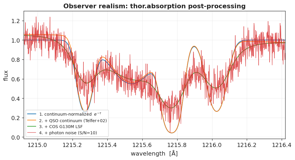
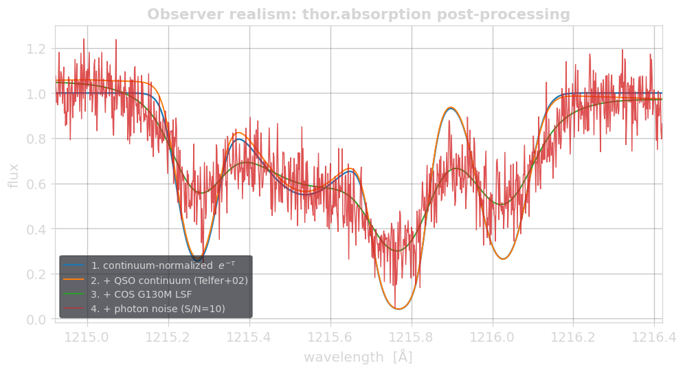
The integrated τ is the physical prediction. To compare with a real spectrograph, the thor.absorption Python package layers on observer effects, each step returning self so they chain:

from thor.absorption import Sightline, Instrument, SpectrumPostProcessor

spec = Sightline("thor_sightline_clumps.zr").spectrum(ray_id=0)   # (lam, tau)
pp = (
    SpectrumPostProcessor(spec)
    .add_qso("qso_telfer2002")        # QSO continuum
    .add_mw_fg("mw_fg_danforth2016")  # Milky-Way foreground (optional)
    .apply_lsf(Instrument("COS-G130M"))
    .add_noise(snr=10, seed=7)
)
pp.save("mock_spectrum.fits")

At this narrow Lyα window the COS LSF is far smaller than the line widths, so it barely smooths the profile; photon noise dominates the difference. Over a broad multi-line spectrum the LSF and QSO-continuum shape matter much more.

Reading the output

SightlineOperator writes a flat/dense layout under sightlines/<savename>/ (default default): a shared wavelength grid plus a dense τ array, with optional per-cell field arrays addressed by a cell_offsets index array. Because each ray crosses a different number of cells, the per-cell fields are stored as one flat array indexed by offsets (the compressed-sparse-row (CSR) layout): ray i's cells occupy [cell_offsets[i], cell_offsets[i+1]), and the last ray runs to the end of the array.

The Sightline loader resolves all of this (the ray_id → row lookup, the CSR slicing, and the (lam, tau) Spectrum), so analysis code never indexes the raw arrays by hand:

import numpy as np
from thor.absorption import Sightline

sl = Sightline("thor_sightline_clumps.zr")
lam, tau = sl.lam, sl.tau(ray_id=0)     # integrated spectrum
cells = sl.fields(ray_id=0)             # {'density','temperature','velocity_x',...}
dl = sl.dl(ray_id=0)                    # per-cell path length (box units)

# velocity-space view, matching the convention above
v_obs = (lam - 1215.67) / 1215.67 * 2.99792458e5   # km/s; blueshift < 0

Trident interoperability

THOR can stand in for Trident for sightline absorption: it integrates τ directly on the native simulation mesh (GPU-accelerated via SYCL), so the thor.absorption pipeline above is usually all you need. When you specifically want Trident's background source spectra (QSO continuum, Milky-Way foreground) or its instrument models, to_trident_spectrum_generator hands you a live trident.SpectrumGenerator with THOR's τ already loaded. From there it is plain Trident, and every normal Trident spectrum method works on the returned object:

from thor.absorption import Sightline, to_trident_spectrum_generator

spec = Sightline("thor_sightline_clumps.zr").spectrum(ray_id=0)
sg = to_trident_spectrum_generator(spec)   # a trident.SpectrumGenerator, τ already loaded

# ...from here, just use Trident as usual:
sg.add_qso_spectrum()              # Trident's QSO background
sg.add_milky_way_foreground()      # Trident's MW foreground
sg.apply_lsf(function="boxcar", width=3)  # explicit LSF; width is in bins
sg.add_gaussian_noise(30)
sg.save_spectrum("spectrum.h5")    # or sg.plot_spectrum("spectrum.png")

Trident is an optional, self-installed dependency (pip install trident); THOR does not bundle it.

Examples

Three worked examples take the same operator from the toy clumps above to a cosmological box: a Lyα forest through TNG50-4, a mock quasar spectrum built from a long skewer, and metal-line CGM absorption through an AGORA galaxy.

A real Lyα forest: TNG50-4

The same operator scales straight to a cosmological box. Here it traces a 512×512 grid of sightlines along +x through the full TNG50-4 snapshot at z = 0 (35 Mpc/h, ≈ 51.7 pMpc, ~18.5 million Voronoi gas cells). The neutral-hydrogen density comes straight from the snapshot's NeutralHydrogenAbundance (THOR derives HIdensity natively, so HI needs no Cloudy table), and Hubble flow is on, so every sightline yields a genuine Lyα forest.

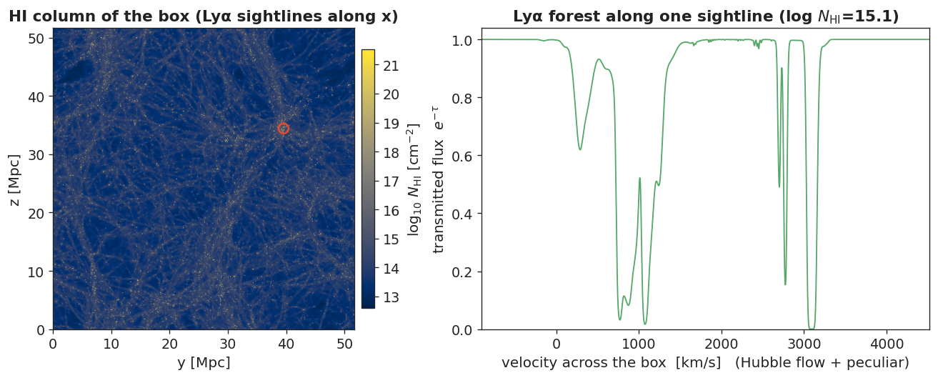
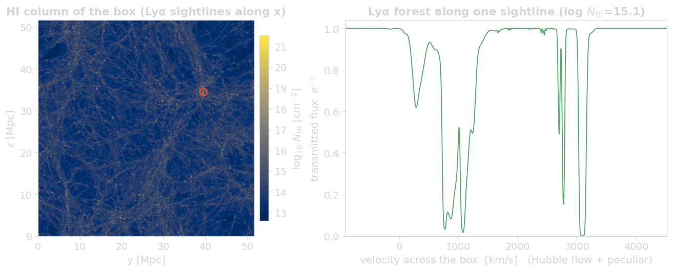
Left: the HI column of every sightline (Σ n_HI · dl) reshaped to the camera grid, the cosmic web in N_HI, with bright high-column systems (Lyman-limit and damped-Lyα absorbers in collapsed halos) threading a diffuse IGM. Right: the transmitted flux along the circled sightline. This is the picture the toy example only stood in for: absorbers at different distances along the box appear at different velocities (distance maps to recession velocity through Hubble flow), from shallow IGM ripples to a saturated system, spread across the ~3500 km/s the box subtends.

Nothing about the operator changed, only the dataset and the density routing:

dataset_type: 'pointcloud_voronoi'        # build a Voronoi mesh on the gas cells
pointcloud_voronoi:
  construction:
    ghost_thickness: 0.1                  # periodic ghost shell as a box fraction; the
                                          # default 0.51 ≈ full replication and OOMs at 18.5M cells
  loader: gadget
  gadget:
    path: /path/to/TNG50-4_snapshot
    fields: ["PositionX", "PositionY", "PositionZ", "Temperature", "Density",
             "VelocityX", "VelocityY", "VelocityZ", "HIdensity"]
raytracer:
  pbc: true                               # true periodic Voronoi
  hubble_flow: 67.74                       # H0 [km/s/Mpc] = h·100 at z=0 → the forest
  operators:
    sightlines:
      ray_source: { type: camera_plane, npixels: [512, 512], direction: [1.0, 0.0, 0.0], length: 1.0 }
      fields: ["HIdensity"]
      tau:
        lines: ['Lya']
        line_density_fields: { Lya: HIdensity }   # integrate n_HI, not the gas mass density
        lambda_min: 1212.0
        lambda_max: 1234.0
        nbins: 2048

Building a mock QSO spectrum

A single box crossing samples a short path. To synthesize a full quasar sightline, i.e. a long Lyα forest blueward of the QSO's Lyα emission, fire the ray at an oblique angle and let it wrap through the periodic box many times (length: 10 box units, pbc: true). With an incommensurate direction each wrap threads fresh structure, so the ray accumulates a long forest spanning the box's Hubble flow (~10 × 3500 km/s, i.e. Δz ≈ 0.12 here). Integrating the Lyman series (Lyα–Lyε) plus the Lyman continuum in one pass gives the Lyα forest, the Lyβ forest, and the Lyman-limit break together. Treat the far end as a quasar at that redshift and multiply the forest transmission exp(−τ) by the qso_telfer2002 QSO continuum (redshifted to z_qso):

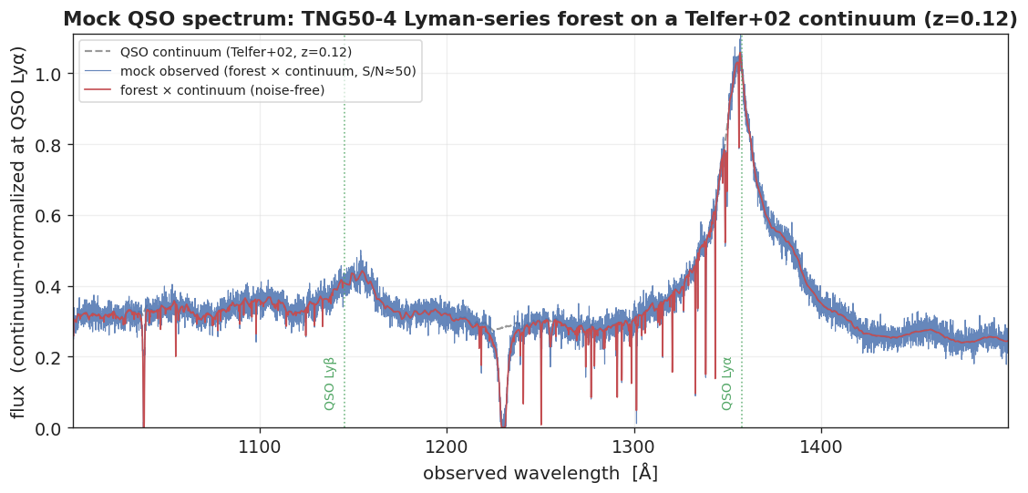
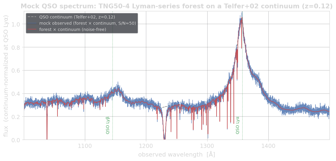
Redward of the QSO Lyα emission peak (~1358 Å) the spectrum is bare continuum. Blueward lies the Lyα forest, and blueward of the QSO Lyβ peak (~1147 Å) the same absorbers reappear as the weaker Lyβ forest.

raytracer:
  pbc: true
  hubble_flow: 67.74
  operators:
    sightlines:
      ray_source:
        type: camera_plane
        direction: [0.892, 0.383, 0.241]    # oblique → fresh structure on each periodic wrap
        length: 10.0                         # ~10 box crossings of forest
      fields: ["HIdensity"]
      tau:
        lines: ['Lya', 'Lyb', 'Lyc', 'Lyd', 'Lye']         # Lyman series
        line_density_fields:
          Lya: HIdensity
          Lyb: HIdensity
          Lyc: HIdensity
          Lyd: HIdensity
          Lye: HIdensity
        include_lyman_continuum: true        # Lyman-limit break
        ll_density_field: HIdensity
        lambda_min: 1000.0
        lambda_max: 1500.0
        nbins: 8192

import numpy as np
from importlib.resources import files
from thor.absorption import Sightline

spec = Sightline("tng_qso.zr").spectrum(ray_id=7)        # (lam, tau) of the long skewer
z_qso = 0.12                                             # far end of the ray
tpl = np.loadtxt(files("thor.absorption") / "data" / "spectral_templates" / "qso_telfer2002.txt")
continuum = np.interp(spec.lam / (1 + z_qso), tpl[:, 0], tpl[:, 1])
mock_flux = continuum * np.exp(-spec.tau)               # QSO continuum × forest

Metal lines: CGM absorption through an AGORA galaxy

THOR derives O VI, C IV and Si IV densities from Cloudy tables using each gas cell's density, temperature, redshift and metallicity. This example traces one sightline through the AGORA z = 4 GIZMO galaxy, excluding star-forming gas from the ion densities.

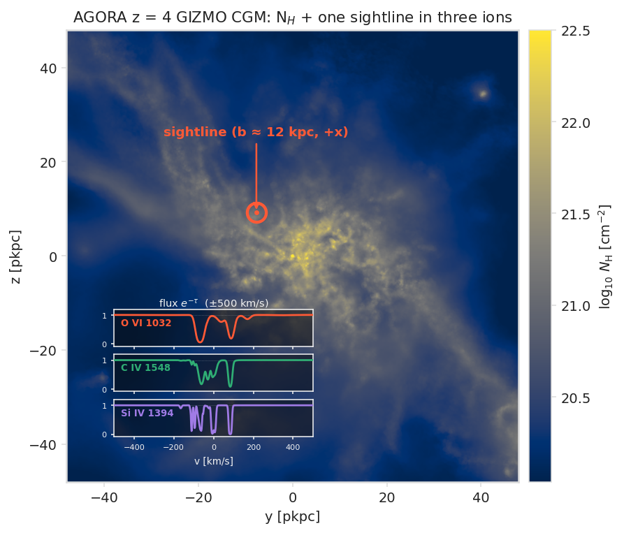
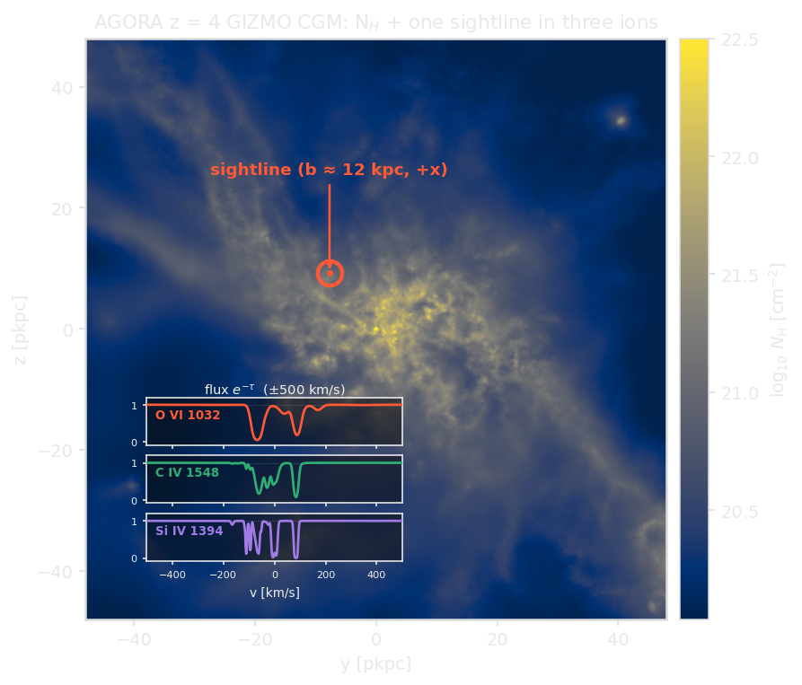
The marked sightline passes about 12 pkpc from the centre. The insets show transmitted flux for O VI 1032, C IV 1548 and Si IV 1394, integrated in one pass.

To reproduce the figure, download the published Cloudy C17.03 v2 ion table and emission table (checksums). Both files are required by the Cloudy reader. Unpack them with:

xz -dc cloudy-c17.03-fg11-rahmati2013-lg-v2-grid_ions.hdf5.xz.part0000 > grid_ions.hdf5
xz -dc cloudy-c17.03-fg11-rahmati2013-lg-v2-grid_emissivities.hdf5.xz.part0000 > grid_emissivities.hdf5

Download the sightline configuration, map configuration and plotting script. Save the shared plotting helper as thorplot.py alongside the plotting script. Set the snapshot and table paths in the YAML files, using the AGORA GIZMO snapshot_152.hdf5 at z = 4, then run from their download directory:

OMP_NUM_THREADS=8 ACPP_VISIBILITY_MASK=omp thor cloudy17-strong-lines.yaml
OMP_NUM_THREADS=8 ACPP_VISIBILITY_MASK=omp thor projection.yaml
python plot.py

The plotting script requires NumPy, Matplotlib and Zarr and writes result.png and result_dark.png. A six-line configuration also includes the weaker doublet members.

See Also

• Ray Tracer Driver: the full sightline configuration (ray sources, multi-line and per-species τ, Hubble modes, MPI, per-cell field selection).
• Datasets Reference: unigrid and pregridded loaders.
• Absorption Lines: THOR vs Trident benchmark (accuracy and throughput) for HI Lyα sightlines through TNG50-4.
• Coherence Length: the related tracer operator, which logs field properties (rather than τ) along rays.