Tracing many sightlines at once
Compare C IV, Si IV and O VI along nine sightlines, then map their strength and velocity across a 64 × 64 grid. The two runs are independent; neither needs output from the single-sightline tutorial or the projection tutorial.
Before you start
Set up the thor command using the installation guide.
Download the galaxy cutout and ionization tables into your working directory. Use the plotting setup, and download thorplot.py beside the plotting scripts. The first metal-absorption tutorial explains how to interpret a single spectrum.
1. Compare nine sightlines
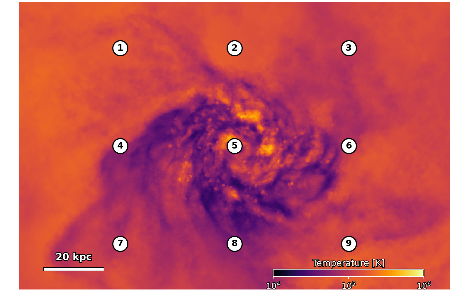
Each numbered dot marks a ray along +z. The spectra below follow the same arrangement; ray 4 matches the single-sightline tutorial.
Download absorption-metals-grid.yaml
and plot_absorption_metals_grid.py.
The complete configuration traces nine parallel rays and writes
to absorption-metals-grid.zr. Each ray uses the same ionization tables.
thor absorption-metals-grid.yaml
uv run --python 3.11 --with zarr --with numpy --with matplotlib plot_absorption_metals_grid.py
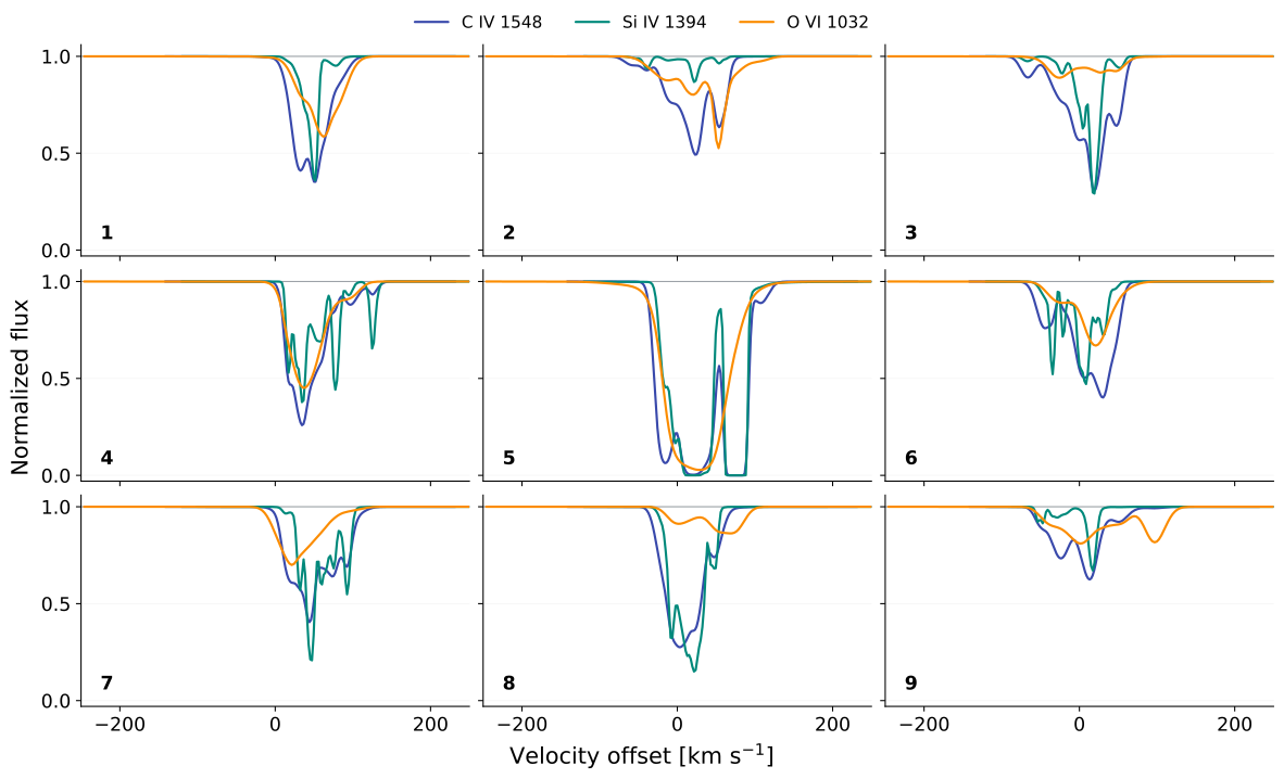
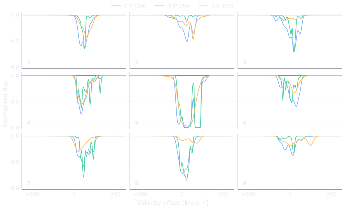
The output image absorption-metals-grid.png compares the nine sightlines.
Both the absorption strengths and the velocity components change between
the central ray (5) and the outer rays.
2. Map absorption with a denser grid
Reuse the cutout and ionization tables. This run does not read the nine-ray output.
Trace a 64 × 64 grid (4,096 rays) across the central 102 × 102 kpc, about 1.6 kpc per pixel. Download absorption-metals-map.yaml and plot_absorption_metals_map.py, then run:
thor absorption-metals-map.yaml
uv run --python 3.11 --with zarr --with numpy --with matplotlib plot_absorption_metals_map.py
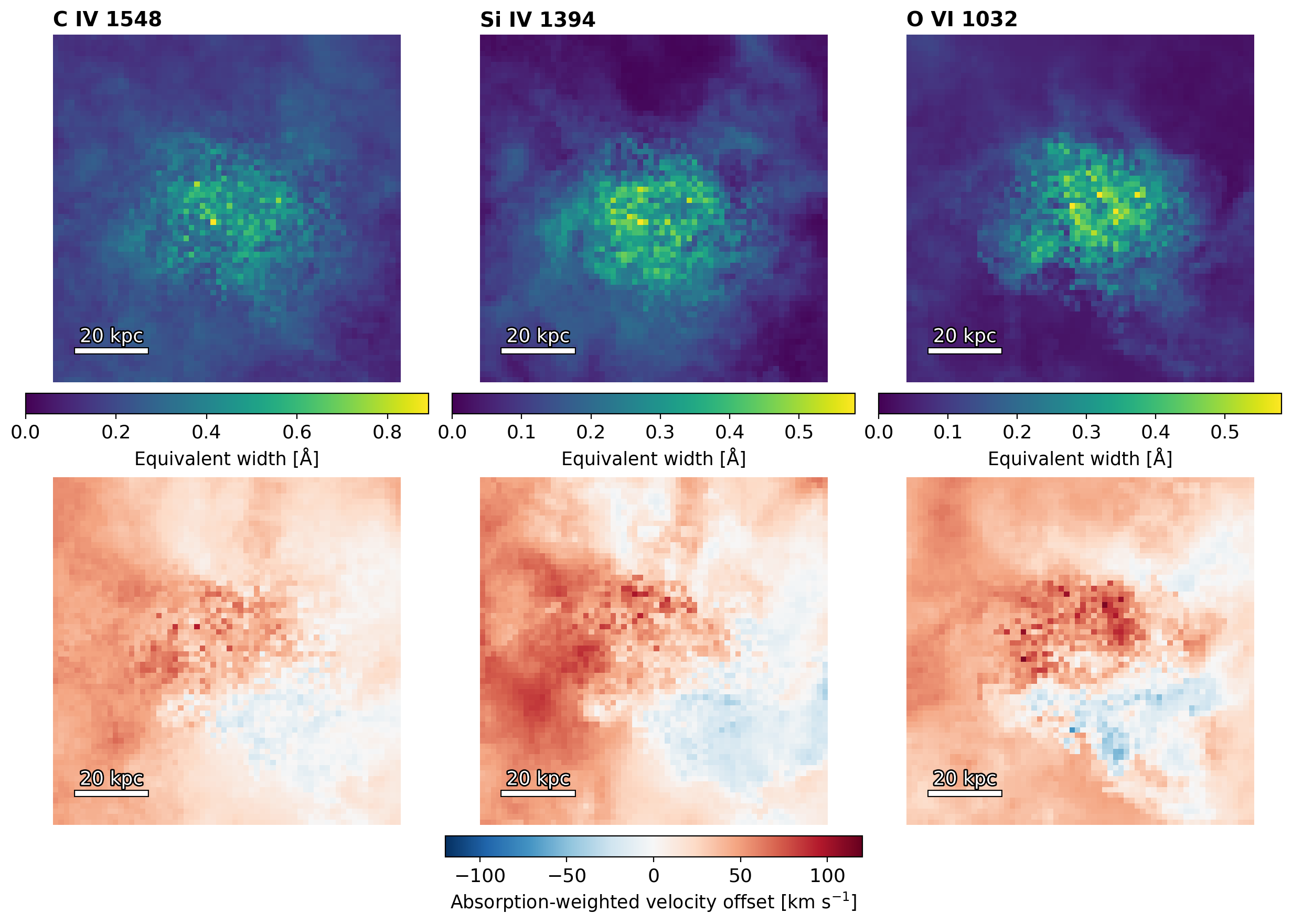
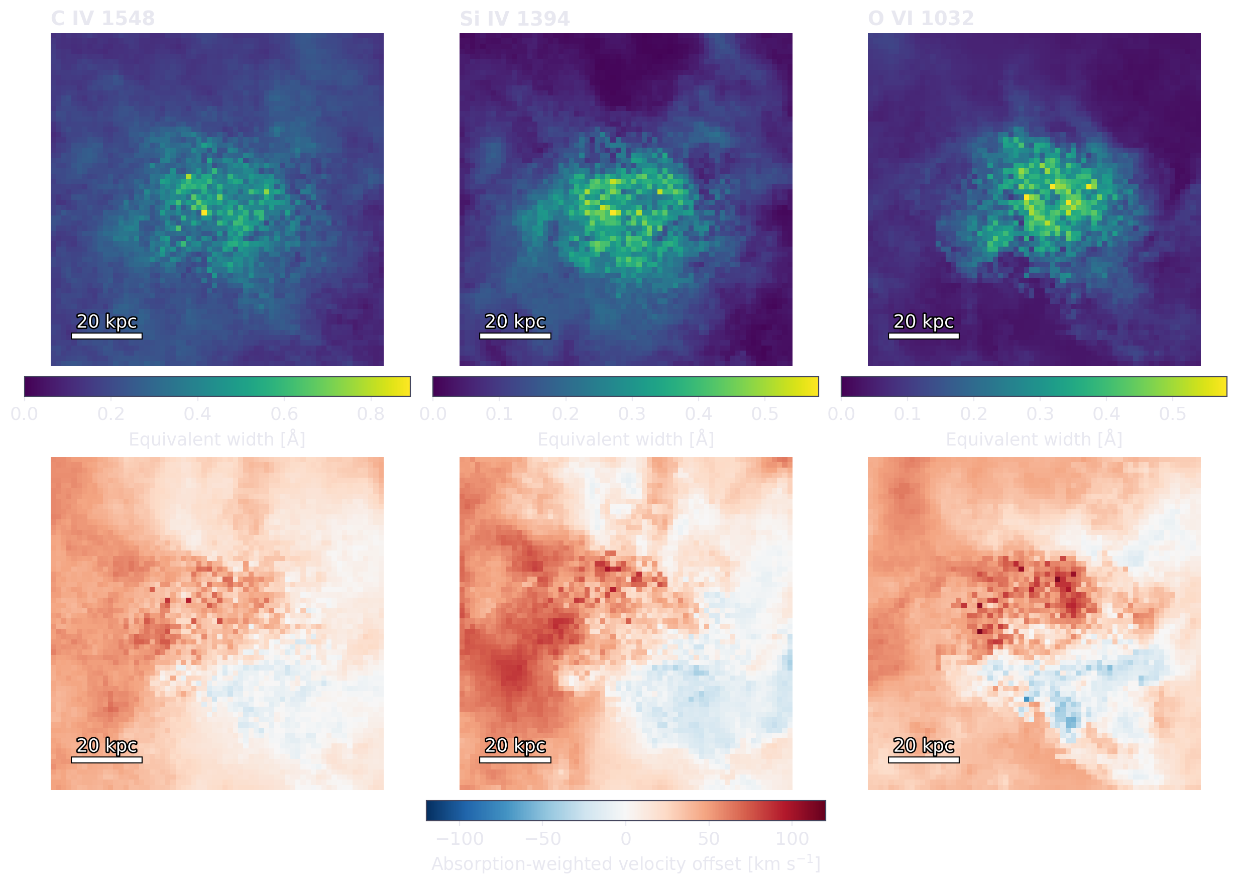
In absorption-metals-map.png, each pixel is one spectrum. The top row shows
equivalent width; the bottom row shows the velocity centroid weighted by the
absorbed fraction \(1-e^{-\tau}\). Blue is blueshifted and red is redshifted,
with the same velocity scale for all three ions. Velocities are relative to
each line's rest wavelength; the galaxy's bulk velocity has not been subtracted.
The maps face the same direction as the temperature projection.