Compare impact parameters and directions
Sample rings around a galaxy, repeat them along several viewing directions, then adapt the configuration to your own galaxy sample.
Before you start
Follow the installation instructions to set up the thor command.
Download the galaxy cutout and ionization tables into your working directory. Use the plotting setup, and download thorplot.py beside the scripts below.
The first two runs use the supplied cutout; the third step requires your own multi-galaxy dataset. For the basic workflow, see the metal-absorption tutorial.
1. Sample rings around the galaxy
Download absorption-metals-rings.yaml
and plot_absorption_rings.py.
Keep thorplot.py in the same directory.
The complete configuration uses these sightline settings:
extent: crossing
ray_source:
  type: impact_parameter
  center: [0.509, 0.489, 0.736]
  direction: [0, 0, 1]
  up: [0, 1, 0]
  impact_parameters: [0, 0.035, 0.07, 0.105]
  n_azimuth: 8
This gives 25 parallel rays: one through the approximate galaxy centre and
eight around each nonzero ring. The centre matches the rotation recipe;
coordinates and radii use the loaded zoom box. One box unit is about 568 kpc.
crossing traces each line from one domain boundary to the other.
thor absorption-metals-rings.yaml
uv run --python 3.11 --with zarr --with numpy --with matplotlib plot_absorption_rings.py absorption-metals-rings.zr
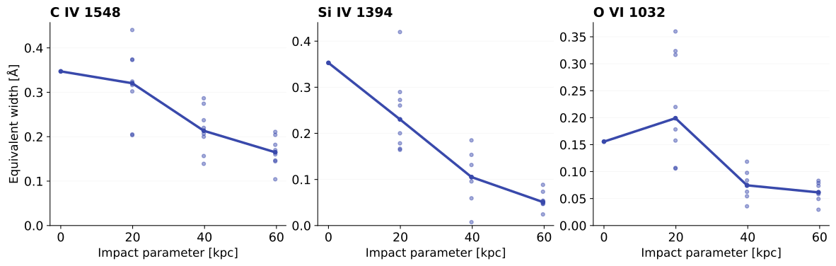
In absorption-metals-rings.png, points show individual rays; lines join
the median equivalent width on each ring. Compare the spread around a ring
with the change between rings. Equal numbers per ring do not sample area uniformly.
2. View the galaxy from several directions
Reuse the inputs and plotting script from step 1. This run does not read the rings output.
Download absorption-metals-views.yaml.
It keeps the same radii and angular sampling, and replaces the source-level
center, direction, and up with:
views:
  type: product
  targets:
    - id: galaxy
      center: [0.509, 0.489, 0.736]
  orientations:
    type: explicit
    frames:
      - id: along_z
        direction: [0, 0, 1]
        up: [0, 1, 0]
      - id: along_x
        direction: [1, 0, 0]
        up: [0, 1, 0]
      - id: inclined
        direction: [1, 0, 1]
        up: [0, 1, 0]
THOR applies every orientation to every target: here, one galaxy × three directions × 25 rays gives 75 spectra. These directions use the simulation's world axes; they are not measured face-on or edge-on disk orientations.
thor absorption-metals-views.yaml
uv run --python 3.11 --with zarr --with numpy --with matplotlib plot_absorption_rings.py absorption-metals-views.zr
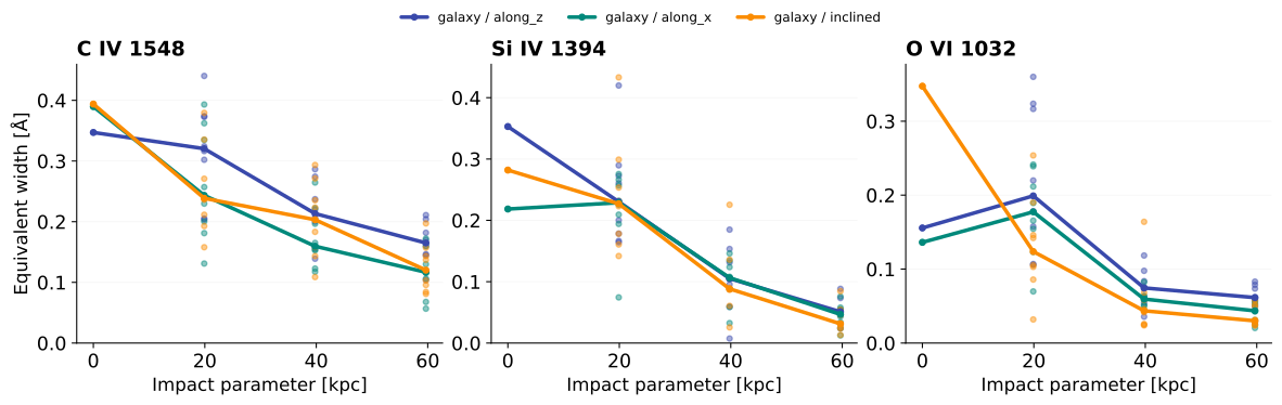
The output image absorption-metals-views.png compares the ring medians between directions.
The +z result matches the rings example. The plotting script groups rays using
view_index and the target/orientation IDs saved in the output.
3. Extend to your own galaxy sample
Adapt absorption-metals-views.yaml from step 2, keeping its orientations and ring pattern.
With your own multi-galaxy snapshot, add each galaxy's centre to targets.
For example, this target list produces 150 rays with the three orientations above:
These are illustrative positions, not two identified galaxies in the tutorial cutout. Use catalogue centres converted to your loaded dataset's coordinates. All targets share that dataset, the radii, and the orientations.
To compare directions relative to each galaxy's disk, add a frame to each
target, with z_axis set to its disk normal and x_axis to an in-plane reference:
These example axes rotate along_z to world +x for halo B. Replace them with
your galaxy's measured axes. Targets without a frame retain world directions.