Resonant line transfer

Learn resonant line transfer by following Lyα photons through a static sphere of neutral hydrogen and plotting the escaping spectrum. Then explore galaxy Lyα and cluster X-ray scattering in the Cookbook examples below.

The first run uses shellmodel with zero inner radius, giving a filled sphere that we can compare with the Dijkstra+06 solution.

1. Configure

From your simulation working directory, download the configuration:

wget https://thor-rt.org/assets/examples/getting-started/my_first_sim.yaml

Until this guide is published, use the preview download.

THOR generates the gas distribution and photon source internally. This example needs no snapshot or reference-table downloads.

This is the complete configuration:

my_first_sim.yaml

dataset_type: 'shellmodel'
driver_type: 'mcrtsimulation'
device: "cpu"
log_level: info

shellmodel:
  boxsize: 3.086e21       # cm (1 kpc)
  inner_radius: 0.0
  outer_radius: 0.1
  density: 0.078098       # cm^-3 (tau ~ 1e6)
  temperature: 20000.0
  density_fluff: 0.0
  temperature_fluff: 0.0
  outflow_velocity: 0.0

mcrtsimulation:
  density_check_lenient: true  # Synthetic density is neutral hydrogen.
  outputpath: output
  overwrite: true
  linename: Lya
  nphotons_max: 10000
  nphotons_step_max: 10000
  nsteps_per_photon_max: 10000000
  acc_scheme: Smith15
  emissionmodel:
    mode: "singlesource"
    singlesource:
      nphotons: 1000
      lum_total: 1e42
      position: [0.5, 0.5, 0.5]

The sphere has radius 100 pc and temperature 20,000 K. Its density gives a center-to-edge line-center optical depth of approximately \(\tau_0=10^6\). The density_check_lenient setting lets this synthetic dataset's density serve as neutral-hydrogen number density. The source emits 1,000 photons.

2. Run

Run from the directory containing the configuration:

thor my_first_sim.yaml

A successful run ends with Thor finished. and its elapsed time. The first container run may take longer while kernels compile. Rerunning this configuration replaces its previous output (overwrite: true).

3. Inspect the result

Download plot_spectrum.py and thorplot.py into your working directory, then run:

uv run --python 3.11 --with h5py --with numpy --with matplotlib plot_spectrum.py

The output image spectrum.png compares the escaping photons with the analytical solution for this static sphere. The plot weights packets by photon rate and normalizes the profile to unit area. For energy-weighted spectra and luminosities, see packet weights.

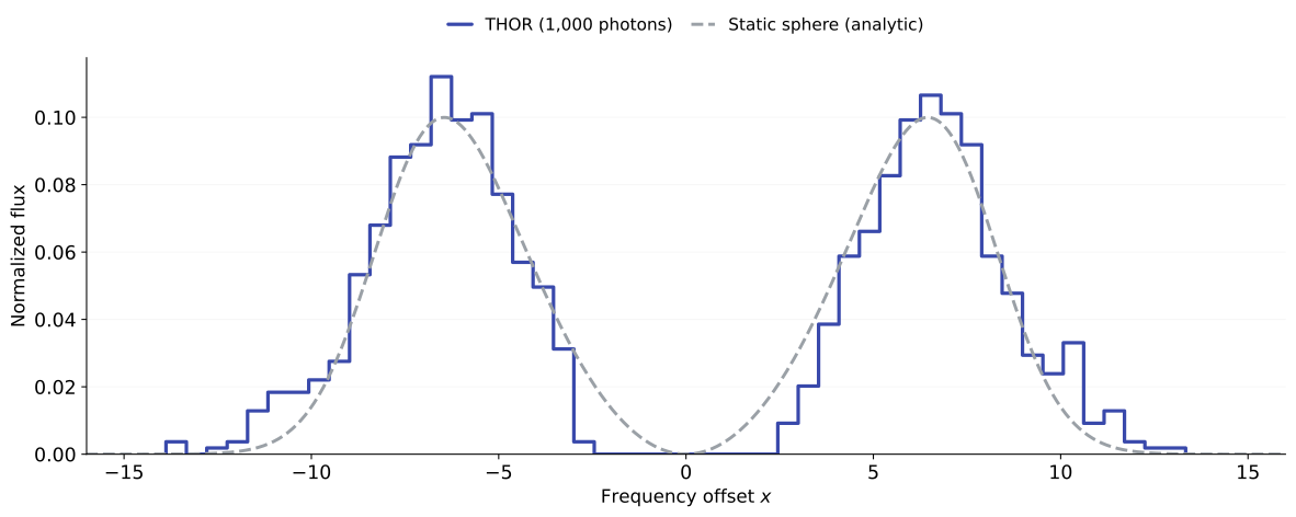
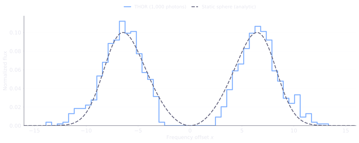
Scattering moves photons away from line center before they escape, producing two peaks. The static sphere gives an approximately symmetric spectrum; with 1,000 photons, individual bins fluctuate around the analytic curve. The horizontal axis is frequency offset in thermal Doppler units; positive values are blueward of line center.

4. Things to try

Increase the optical depthPush the peaks farther apart.

Copy my_first_sim.yaml to denser.yaml and change these values, keeping the other settings:

shellmodel:
  density: 0.78098       # ten times the original density
mcrtsimulation:
  outputpath: output-denser

Run the new configuration:

thor denser.yaml

Download plot_spectrum_variation.py into the same directory and compare with the original run:

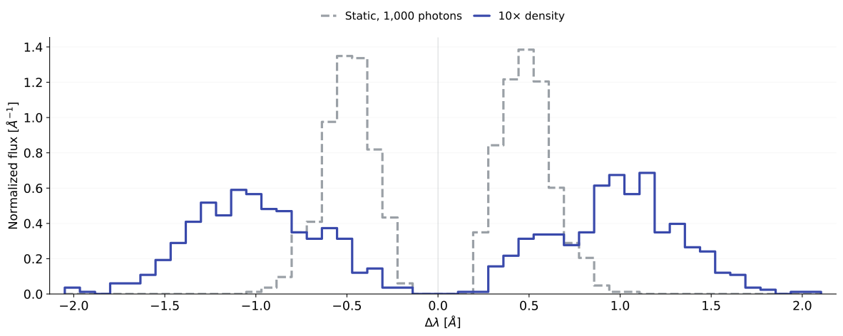
uv run --python 3.11 --with h5py --with numpy --with matplotlib plot_spectrum_variation.py denser

In spectrum-denser.png, both photon-rate profiles use the same bins and are normalized to unit area.

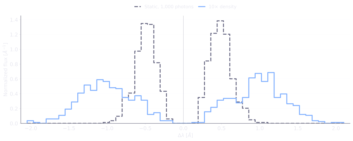
The larger optical depth pushes the peaks farther from line center. In this optically thick limit, offsets scale approximately as \(\tau_0^{1/3}\), so ten times the density increases their separation by about 2.15 times.

With thor-tools, you can also compare with the higher-optical-depth analytic solution:

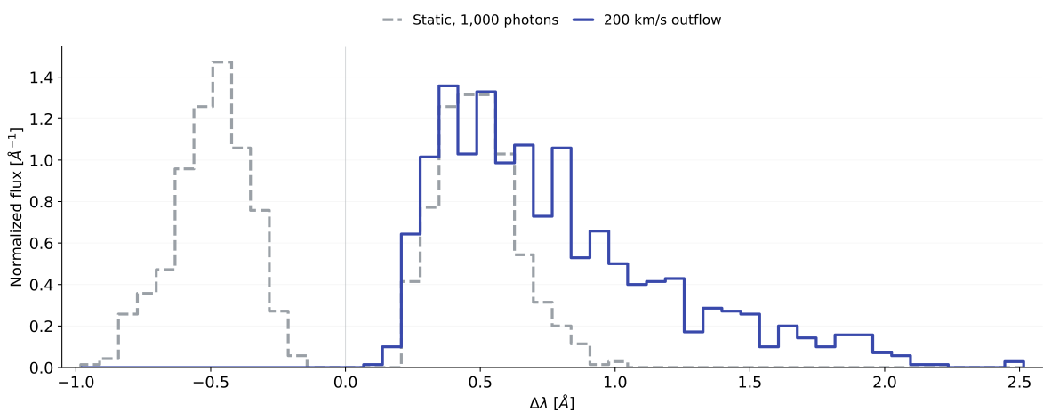
thor-tools mcrt spectrum plot denser.yaml --compare-analytic sphere --tau0 1e7 -o plots-denser

Add an outflowSee how moving gas changes the spectrum.

Copy my_first_sim.yaml to outflow.yaml and change these values:

shellmodel:
  outflow_velocity: 2e7  # cm/s (200 km/s) at the outer radius
mcrtsimulation:
  outputpath: output-outflow
  max_step: 0.00009     # resolve the changing gas velocity

Run the new configuration:

thor outflow.yaml

Download plot_spectrum_variation.py into the same directory and compare with the original run:

uv run --python 3.11 --with h5py --with numpy --with matplotlib plot_spectrum_variation.py outflow

In spectrum-outflow.png, both photon-rate profiles use the same bins and are normalized to unit area.

The small max_step resolves the velocity gradient across the sphere. Expansion makes the spectrum asymmetric, favoring the red side (Δλ > 0). The static-sphere analytic curve no longer applies.

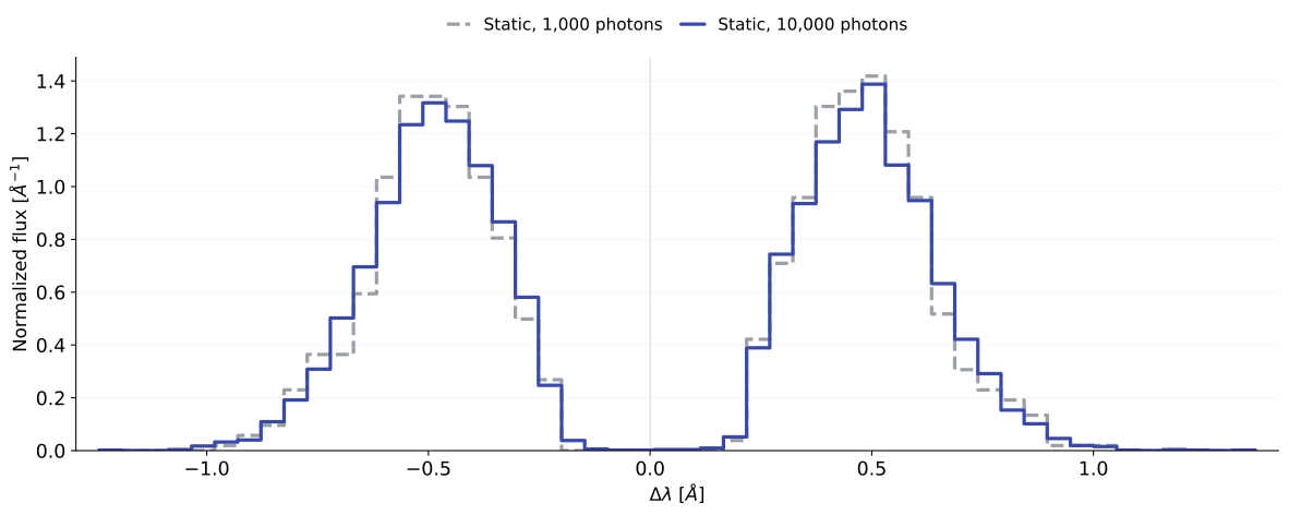
Reduce the noiseMake the spectrum smoother with more photons.

Copy my_first_sim.yaml to smoother.yaml and change these values:

mcrtsimulation:
  outputpath: output-smoother
  emissionmodel:
    singlesource:
      nphotons: 10000

Run the new configuration:

thor smoother.yaml

Download plot_spectrum_variation.py into the same directory and compare with the original run:

uv run --python 3.11 --with h5py --with numpy --with matplotlib plot_spectrum_variation.py smoother

In spectrum-smoother.png, both photon-rate profiles use the same bins and are normalized to unit area.

The spectrum keeps the same overall shape, with smaller sampling fluctuations. Ten times as many photons reduce typical Monte Carlo noise by about \(\sqrt{10}\), while increasing the runtime.

Plot with thor-tools

If you have a THOR checkout, you can also use its analysis CLI:

uv tool install --python 3.11 "/path/to/thor/python/thor-rt[mcrt]"
thor-tools mcrt spectrum plot my_first_sim.yaml --compare-analytic sphere --tau0 1e6

The output image plots/spectrum_original_global.png shows the same analytical comparison. See MCRT analysis for more options.

Continue in the Cookbook

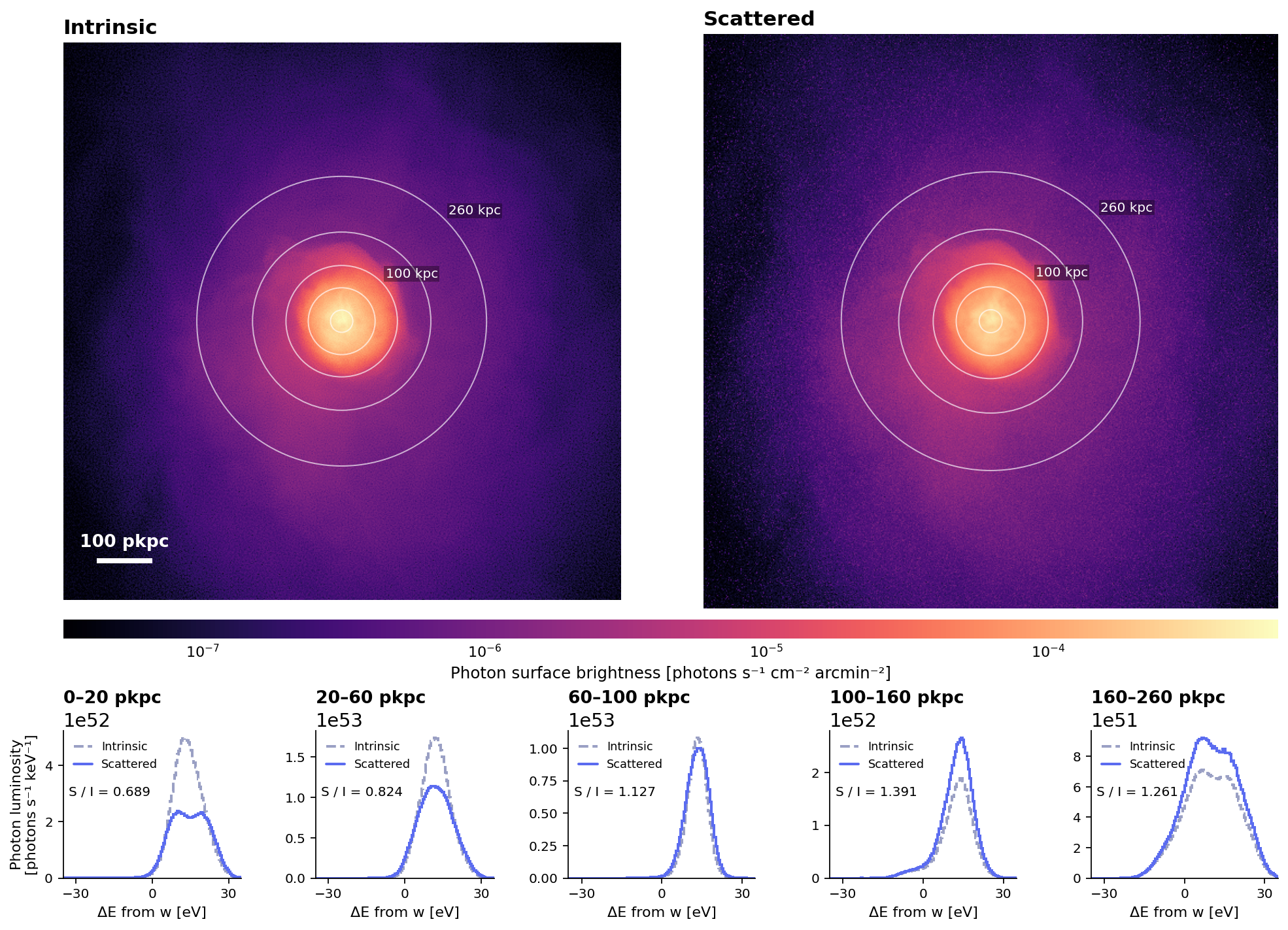
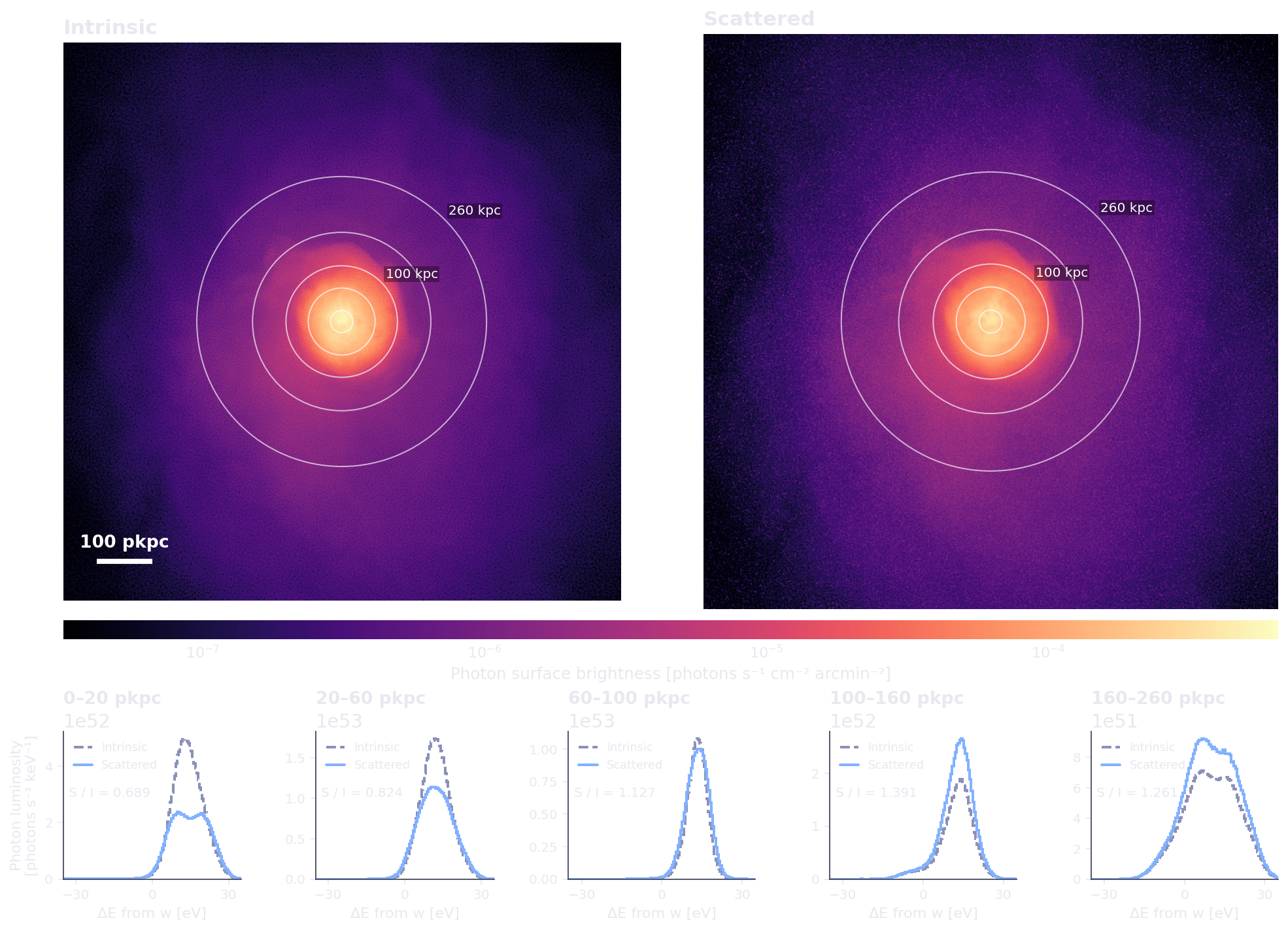
Apply the same workflow to a simulated galaxy or galaxy cluster.