Absorption spectra
Compare C IV, Si IV, and O VI absorption along one ray through the TNG50 cutout. Cloudy tables supply the ion fractions; the snapshot supplies the elemental abundances.
1. Download the configuration
Inputs required
Download the galaxy cutout and ionization tables from Prepare.
Download absorption-metals.yaml into your working directory.
2. Configure and run
absorption-metals.yaml
# Metal absorption using Cloudy C17.03 FG11 v2 tables. [AI-Codex]
dataset_type: pointcloud_voronoi
driver_type: raytracer
device: cpu
log_level: info

pointcloud_voronoi:
  hilbert_bits: 8
  loader: gadget
  cloudy:
    enabled: true
    ion_table_path: ./data/cloudy-v2/grid_ions.hdf5
    emission_table_path: ./data/cloudy-v2/grid_emissivities.hdf5
    redshift_interp: true
  gadget:
    path: ./tng50-halo625-gas-stars-v2.hdf5
    fields: [PositionX, PositionY, PositionZ, Density, Temperature,
             StarFormationRate, VelocityX, VelocityY, VelocityZ,
             cloudydensity_CIV, cloudydensity_SiIV, cloudydensity_OVI]
    zoom_box: [[0.4945, 0.5055], [0.4945, 0.5055], [0.4919, 0.5029]]
  field_filters:
    _non_star_forming:
      conditions:
        - {field: StarFormationRate, op: "==", value: 0.0}
      else: zero
    cloudydensity_CIV: {inherit: _non_star_forming}
    cloudydensity_SiIV: {inherit: _non_star_forming}
    cloudydensity_OVI: {inherit: _non_star_forming}

raytracer:
  max_step: 0.01
  hubble_flow: 0.0
  outputpath: absorption-metals.zr
  overwrite: true
  operators:
    sightlines:
      output:
        cells: true
      rays:
        - {id: 0, start: [0.57, 0.5, 0.01], end: [0.57, 0.5, 0.99]}
      tau:
        lines: [CIV, SiIV, OVI]
        line_density_fields:
          CIV: cloudydensity_CIV
          SiIV: cloudydensity_SiIV
          OVI: cloudydensity_OVI
        per_species: true
        lambda_min: 1028.0
        lambda_max: 1552.0
        nbins: 52400
The ray looks along +z, about 40 physical kpc from the map center. The dot marks its position on the visualization tutorial's temperature map: the ray travels into the image. This reuses the earlier projection; you do not need to render it again.
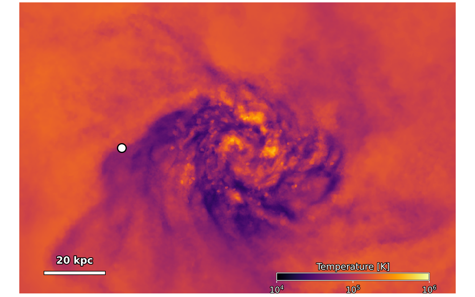
The map shows density-weighted mean temperature along the viewing direction, rather than the depth of individual absorbers.
line_density_fields assigns each transition its own ion number density.
per_species: true saves their optical depths separately for plotting.
THOR multiplies each table ion fraction by the element number density from
GFM_Metals. These absorption lines assume ground-state ions.
The field filters exclude star-forming gas, whose effective temperature is unsuitable for this equilibrium calculation. Hubble flow is off.
A successful run ends with Thor finished. and writes absorption-metals.zr.
Rerunning replaces that output (overwrite: true).
3. Inspect the result
Download thorplot.py and plot_absorption_metals.py into the same directory, then run:
The output image absorption-metals.png
compares the three ions.
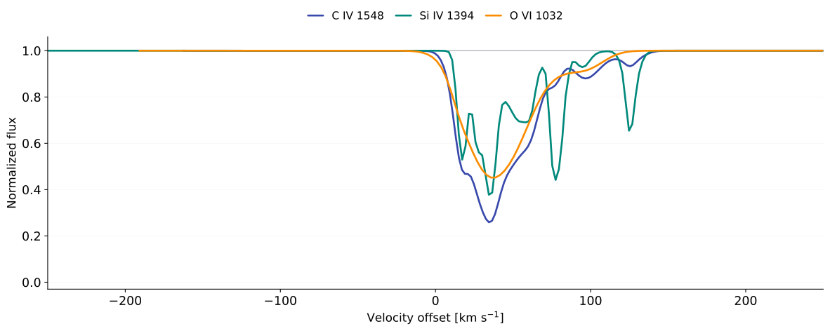
Each curve shows normalized flux \(e^{-\tau}\) against velocity relative to its own rest wavelength: C IV 1548.187 Å, Si IV 1393.755 Å, and O VI 1031.912 Å. The galaxy's bulk velocity has not been subtracted.
The narrow C IV and Si IV components contrast with the broader O VI profile. The ions weight the gas differently through their ion fractions and elemental abundances; their thermal widths also depend on temperature and atomic mass. No instrumental broadening or noise has been added.
4. Things to try
Trace the absorbing gasConnect gas density and velocity to the absorption features.
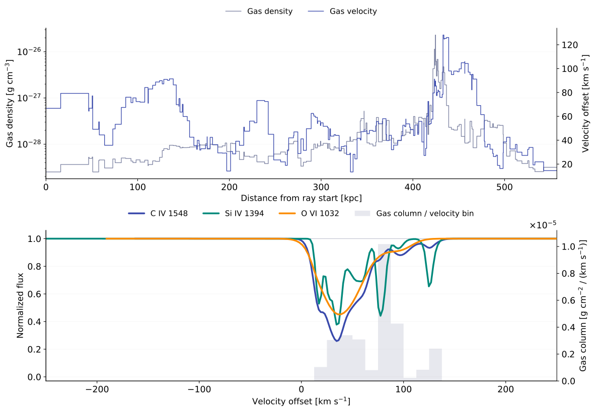
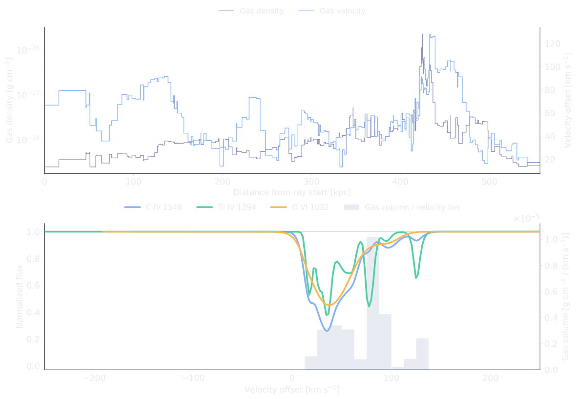
The same run records the density, velocity and path length of each crossed
cell (output.cells: true). No second simulation is needed.
Download plot_absorption_gas.py
beside thorplot.py, then run:
In absorption-gas.png, the top panel shows density and velocity along
the ray. The lower panel overlays gas mass column per velocity bin in gray
on the absorption spectra, using the right axis for its units.
Positive velocity means redshift; gas moving toward the observer has negative velocity.
The gray profile includes all traced gas. Ion fractions, elemental abundances and thermal broadening determine how that gas appears in each absorption line.
Move the sightline
Change 0.57 to 0.61 in both ray endpoints, then run THOR and the plotting
command again. The new ray passes about 63 kpc from the map center, farther left
on the map. Compare which components remain visible in each ion.
Continue in the Cookbook
Extend the single sightline to a grid of spectra and maps of absorption strength.
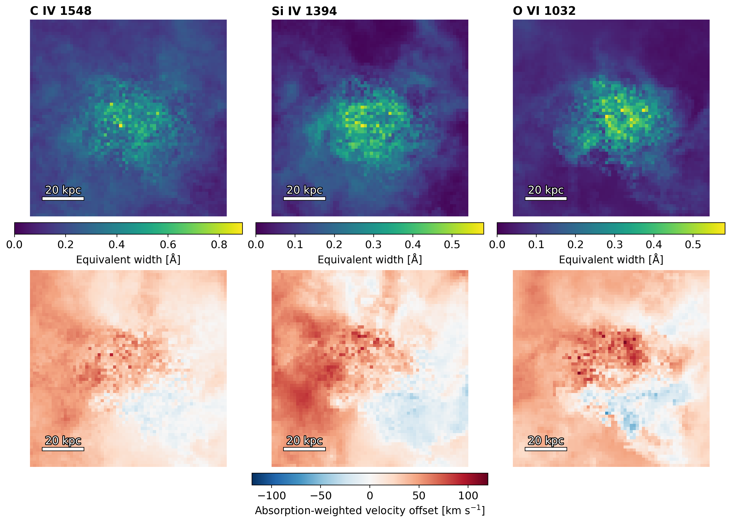
For mock-observation workflows, see Sightline absorption.